Playing with the HEP system of units¶

Or, an intro to the hepunits package while performing some time-of-flight studies.

Warning

The URL for this page may change, the general design for this tutorial series is in flux.

Scikit-HEP packages used:

Authors

Eduardo Rodrigues

import numpy as np
import matplotlib.pyplot as plt

hepunits - The HEP system of units¶

The package hepunits collects the most commonly used units and constants in the HEP System of Units, which differs from the international system of units (aka SI units) by scaling factors for what are the basic units. The HEP system of units is based on the following:

Quantity	Name	Unit
Length	millimeter	mm
Time	nanosecond	ns
Energy	Mega electron Volt	MeV
Positron charge	eplus
Temperature	kelvin	K
Amount of substance	mole	mol
Luminous intensity	candela	cd
Plane angle	radian	rad
Solid angle	steradian	sr

Note: no need to make use of sophisticated packages (e.g. as in AstroPy) since we basically never need to change systems of units (we never use ergs as energy, for example ;-)).

Basic usage¶

Basic usage is straightforward, though it may be confusing at first. Remember, all variables are written wrt to the units:

from hepunits import GeV, MeV, cd, eplus, kelvin, mm, mol, ns, rad, sr

mm == ns == MeV == eplus == kelvin == mol == cd == rad == sr == 1

True

GeV == 1000 * MeV

True

Note

No error checking is implemented, since units are not objects, rather simple numbers. Expressions such as 1*ns + 1*mm produce no error.
Units help improving the readability of code and making formula explicit (although correctness must be still manually checked).

Add two quantities with different length units:

from hepunits import units as u

1 * u.meter + 5 * u.cm

1050.0

The result is in HEP units, so mm. Indeed, for example u.meter == 1000 == 1000 * u.mm.

Rather obtain the result in meters:

(1 * u.meter + 5 * u.cm) / u.meter

1.05

Do you need to play a bit more to get a proper feeling? This next (non-academic) exercise should help you …

Quick time-of-flight study¶

Let’s try to play with units in a meaningful way, in a kind of exercise that physicists encounter. Imagine you are investigating time-of-flight (ToF) detectors for particle identification. The time it takes a particle of velocity \(\beta = v/c= pc/E\) to travel a distance \(L\) is given by

\[\mathrm{ToF} = \frac{L}{c \beta}\]

It results that the mass \(m\) of the particle can be determined from

\[m = \frac{p}{c}\sqrt{\frac{c^2 \mathrm{ToF}^2}{L^2}-1}\]

provided the path length \(L\) and the momentum \(p\) can be measured, say, by a tracking system.

What are typical ToF differences say for (charged) kaons and pions? It is practical to perform the calculation as

\[\Delta \mathrm{ToF} = \frac{L}{c}(\frac{1}{\beta_1} - \frac{1}{\beta_2})\,,\]

with \(\frac{1}{\beta} = \sqrt{1+m^2c^2/p^2}\).

from hepunits import GeV, c_light, meter, ns, ps


def ToF(m: float, p: float, L:float) -> float:
    """Time-of-Flight = particle path length L / (c * β)"""
    one_over_β = np.sqrt(
        1 + m * m / (p * p)
    )  # no c factors here because m and p given without them, hence c's cancel out ;-)
    return L * one_over_β / c_light

For convenience, get hold of data for the proton, \(K^+\) and \(\pi^+\) taken from the PDG using the Particle package:

from particle.literals import K_plus, pi_plus, proton  # particle name literals

Calculate the difference in ToF between 10 GeV kaons and pions travelling over 10 meters:

delta = (
    ToF(K_plus.mass, 10 * GeV, 10 * meter) - ToF(pi_plus.mass, 10 * GeV, 10 * meter)
) / ps

print(f"At 10 GeV, Delta-TOF(K-pi) over 10 meters = {delta:.4} ps")

At 10 GeV, Delta-TOF(K-pi) over 10 meters = 37.37 ps

Let’s get a bit fancier:

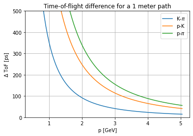
Compare protons, kaons and pions.
Look at the ToF difference versus momentum.

p = np.arange(0.5, 5.1, 0.05) * GeV

delta1 = (ToF(K_plus.mass, p, 1.0 * meter) - ToF(pi_plus.mass, p, 1.0 * meter)) / ps
delta2 = (ToF(proton.mass, p, 1.0 * meter) - ToF(K_plus.mass, p, 1.0 * meter)) / ps
delta3 = (ToF(proton.mass, p, 1.0 * meter) - ToF(pi_plus.mass, p, 1.0 * meter)) / ps

fig, ax = plt.subplots()
ax.plot(p / GeV, delta1, label="K-$\pi$")
ax.plot(p / GeV, delta2, label="p-K")
ax.plot(p / GeV, delta3, label="p-$\pi$")

ax.set(
    xlabel="p [GeV]",
    ylabel="$\Delta$ ToF [ps]",
    title="Time-of-flight difference for a 1 meter path",
)
ax.grid()

plt.legend()
plt.ylim(bottom=0, top=500)
plt.show()

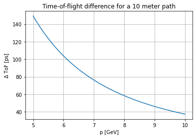
Taking now an example that could be relevant to LHCb conditions - detector timing resolution requirement is getting tough!:

p = np.arange(5.0, 10.1, 0.1) * GeV
delta = (ToF(K_plus.mass, p, 10 * meter) - ToF(pi_plus.mass, p, 10 * meter)) / ps

fig, ax = plt.subplots()
ax.plot(p / GeV, delta)

ax.set(
    xlabel="p [GeV]",
    ylabel="$\Delta$ ToF [ps]",
    title="Time-of-flight difference for a 10 meter path",
)
ax.grid()

plt.show()

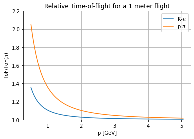
For short flight distances protons, kaons and pions become indistinguishable, as expected:

p = np.arange(0.5, 5.1, 0.05) * GeV
s1 = ToF(K_plus.mass, p, 1.38 * meter) / ToF(pi_plus.mass, p, 1.38 * meter)
s3 = ToF(proton.mass, p, 1.38 * meter) / ToF(pi_plus.mass, p, 1.38 * meter)

fig, ax = plt.subplots()
ax.plot(p / GeV, s1, label="K-$\pi$")
ax.plot(p / GeV, s3, label="p-$\pi$")

ax.set(
    xlabel="p [GeV]",
    ylabel="ToF/ToF($\pi$)",
    title="Relative Time-of-flight for a 1 meter flight",
)
ax.grid()

plt.ylim(bottom=1, top=2.2)
plt.legend()
plt.show()

Scikit-HEP Tutorials

Playing with the HEP system of units

Contents

Playing with the HEP system of units¶

hepunits - The HEP system of units¶

Basic usage¶

Quick time-of-flight study¶

Playing with the HEP system of units¶

hepunits - The HEP system of units¶

Basic usage¶

Quick time-of-flight study¶