Basic Plotting¤
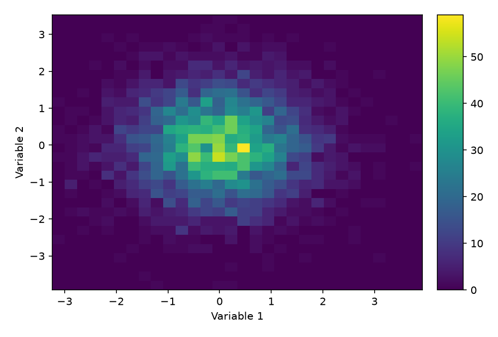
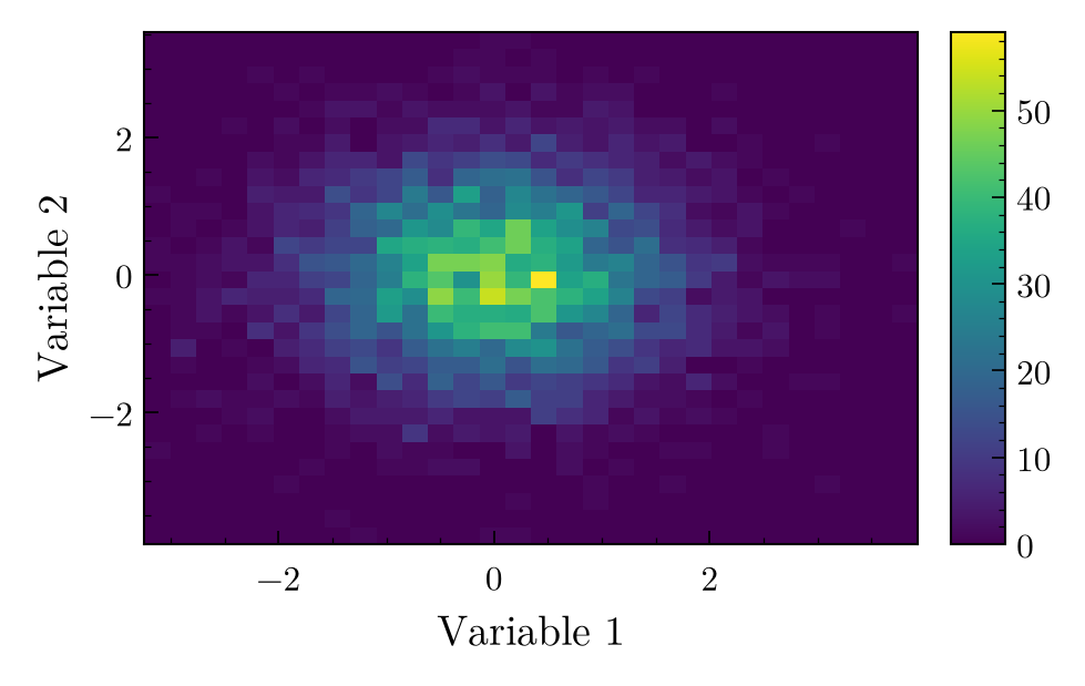
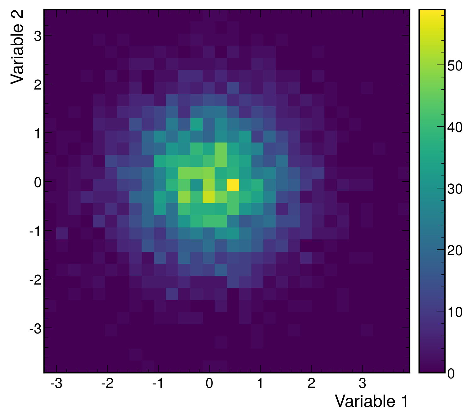
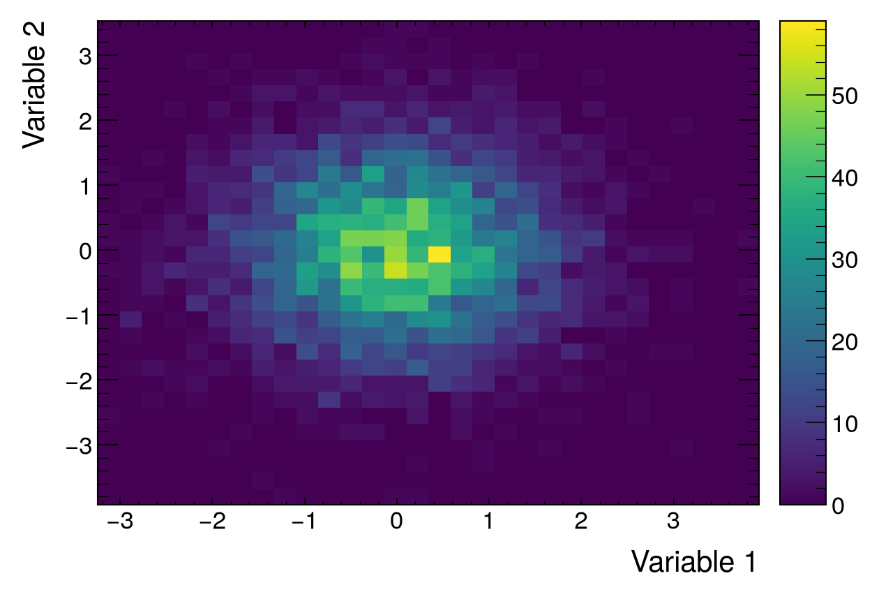
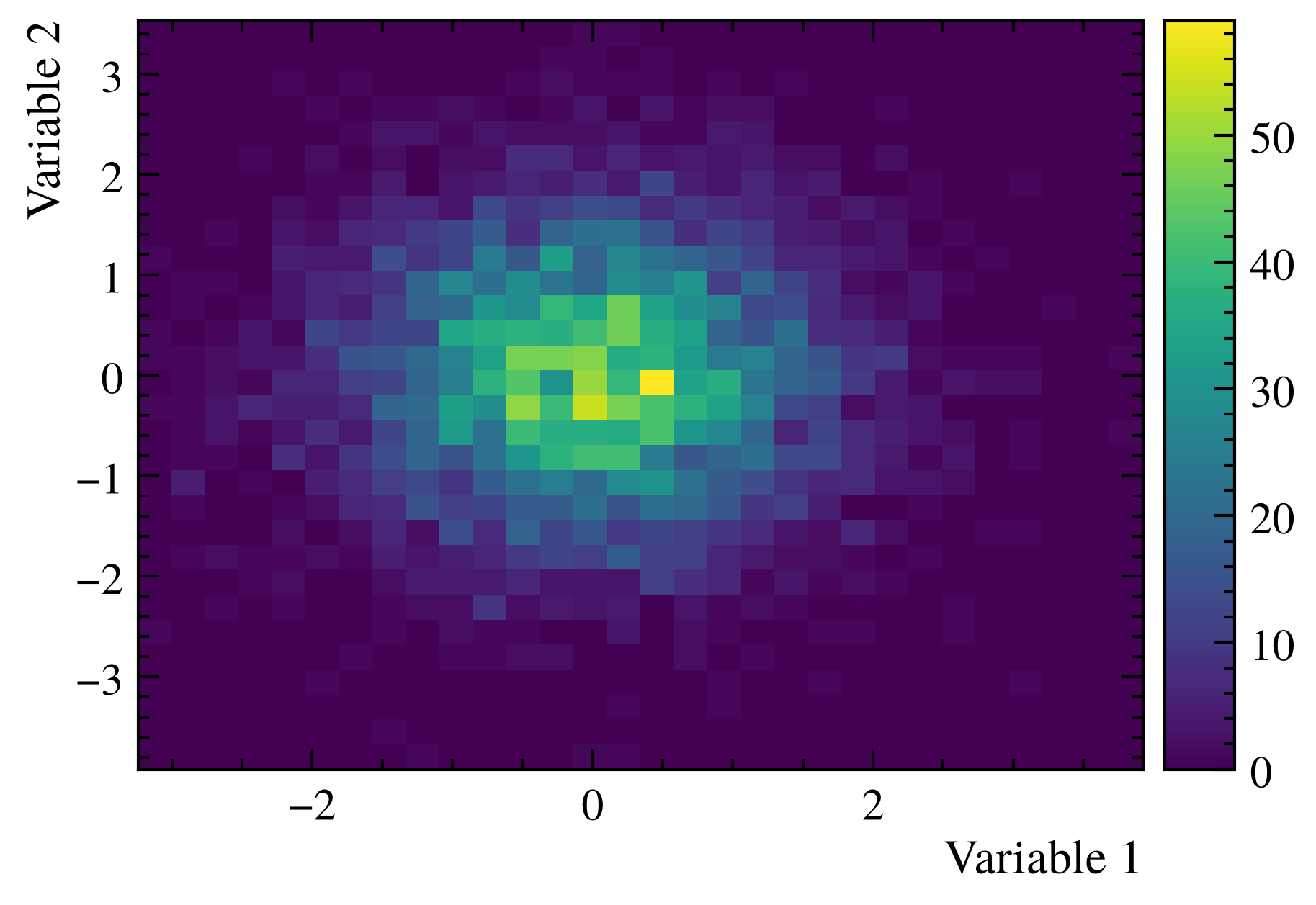
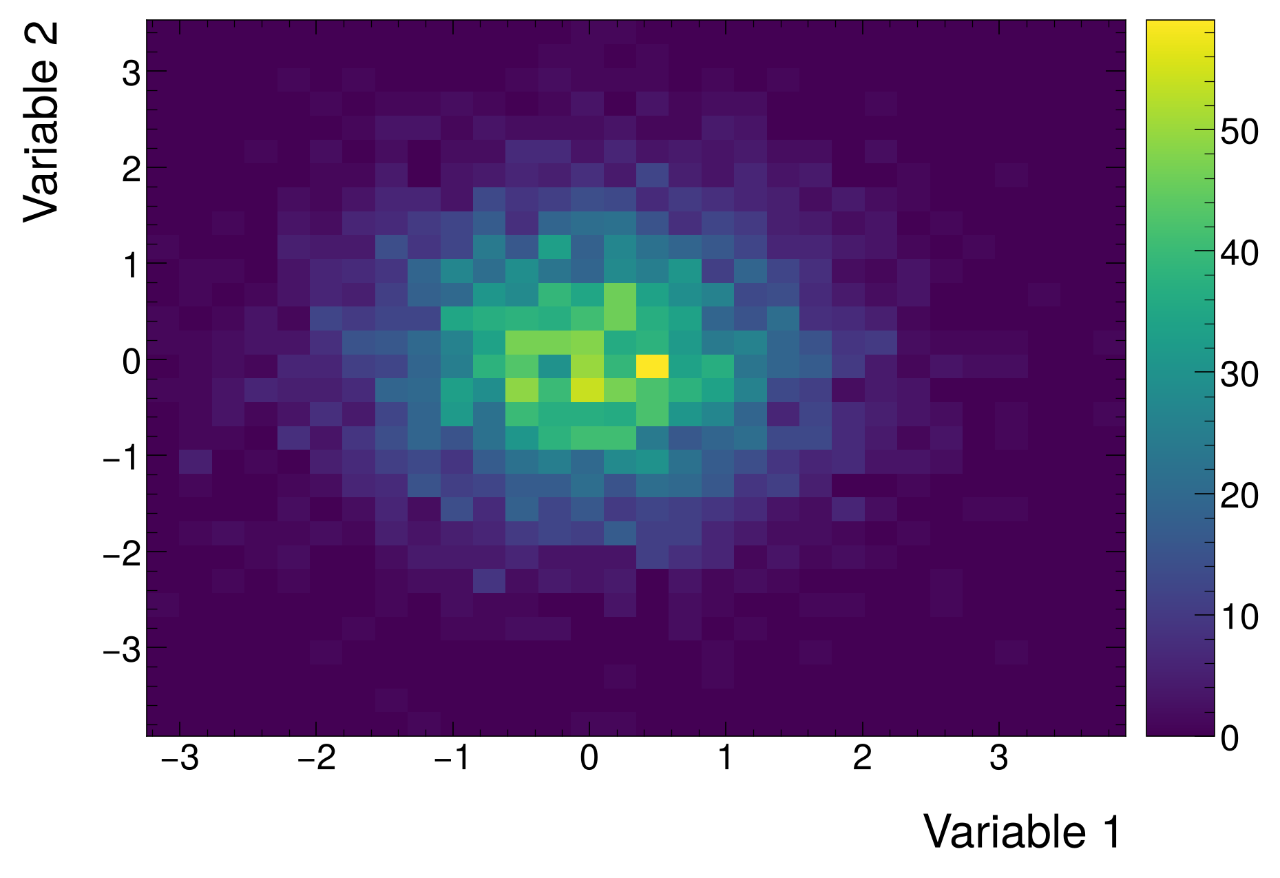
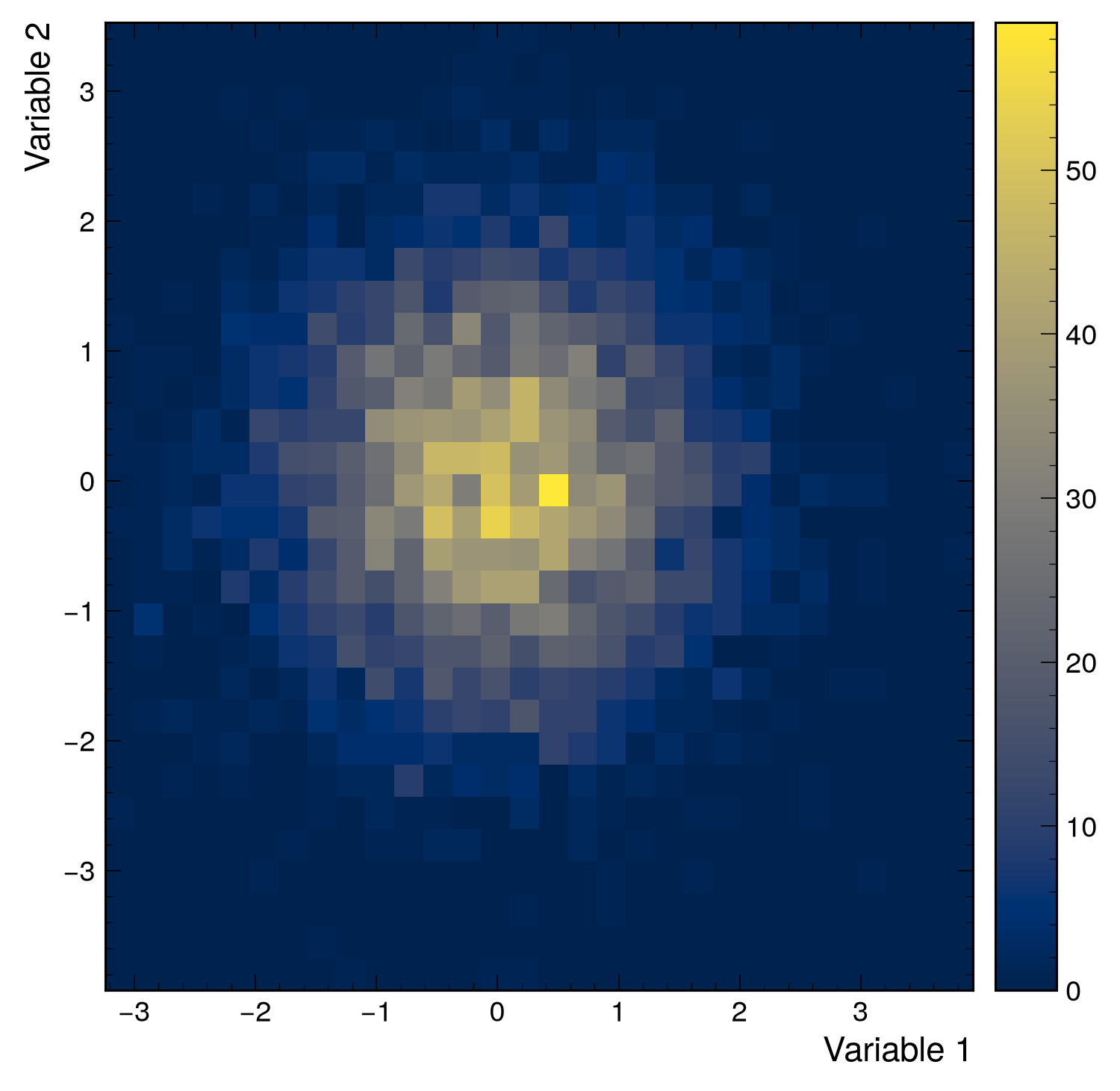
This section covers the core plotting functionality of mplhep for plotting 1D and 2D histograms.
Prerequisites
Throughout this guide the following codeblock is assumed.
1D Histogram Plotting¤
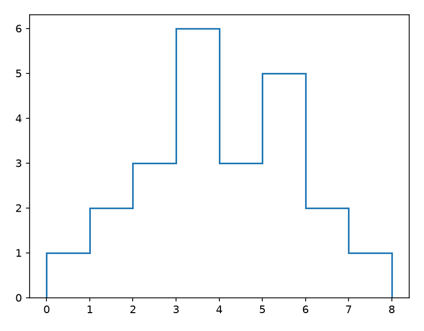
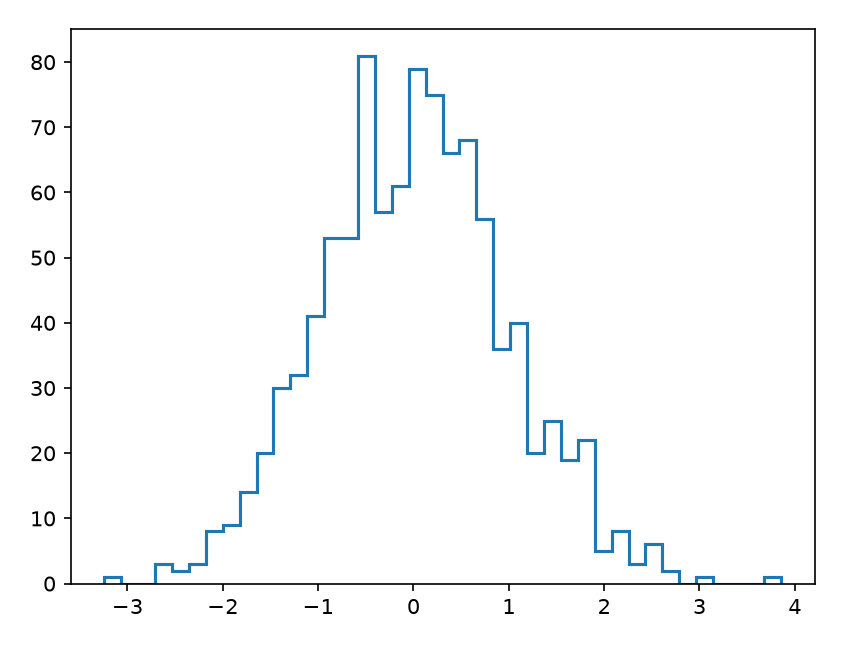
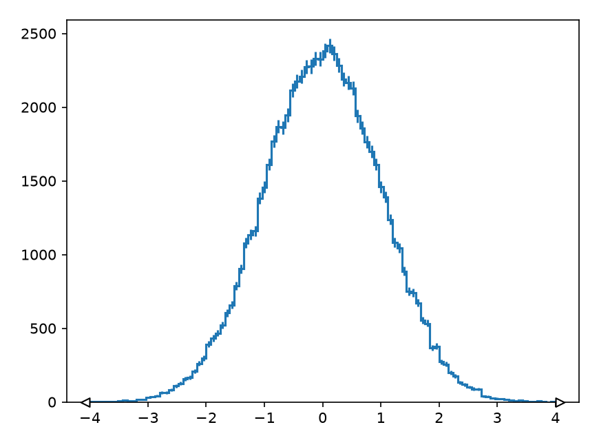
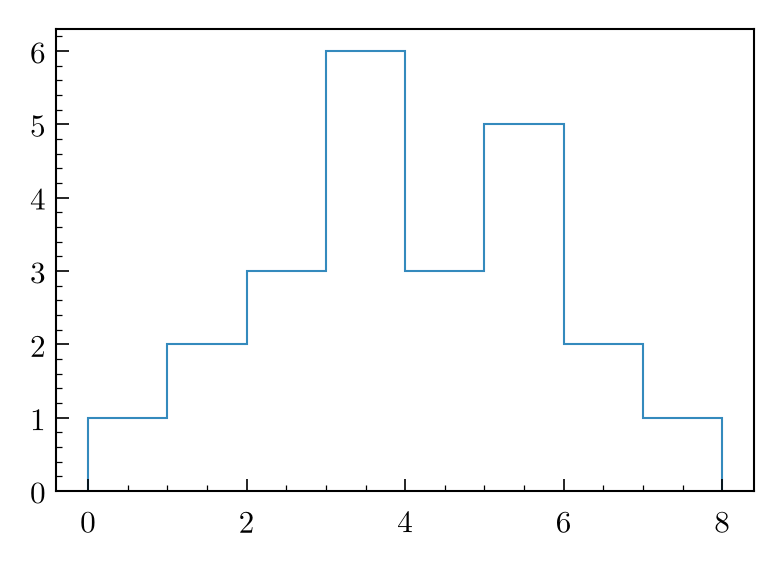
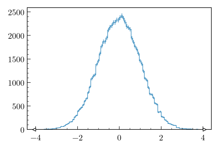
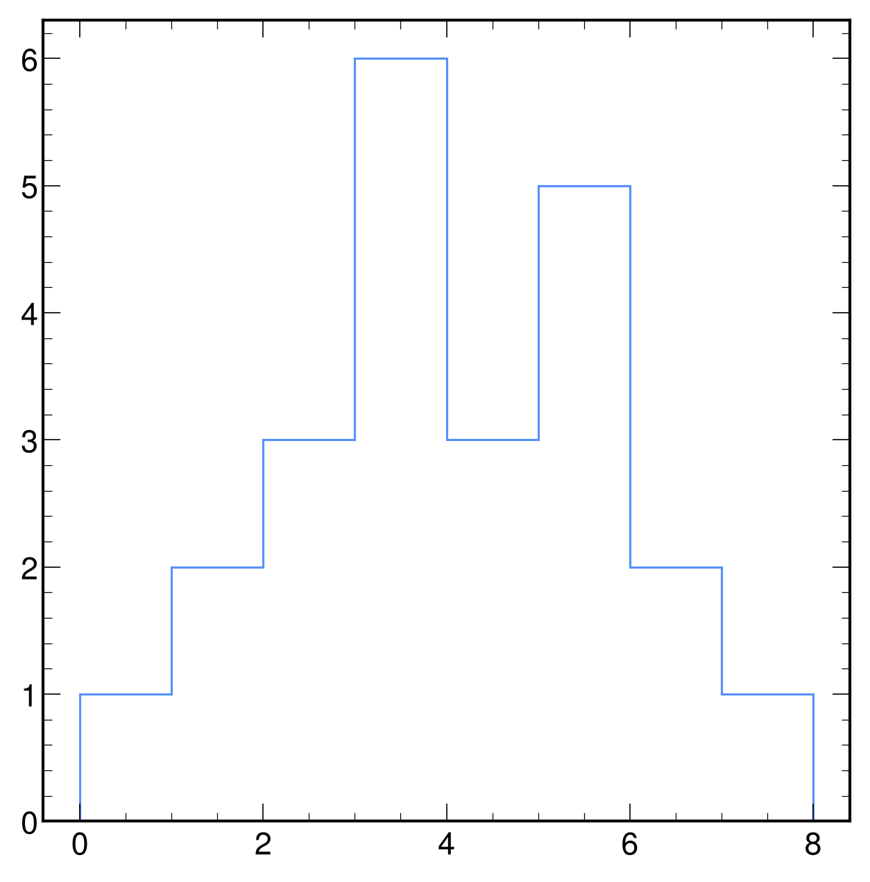
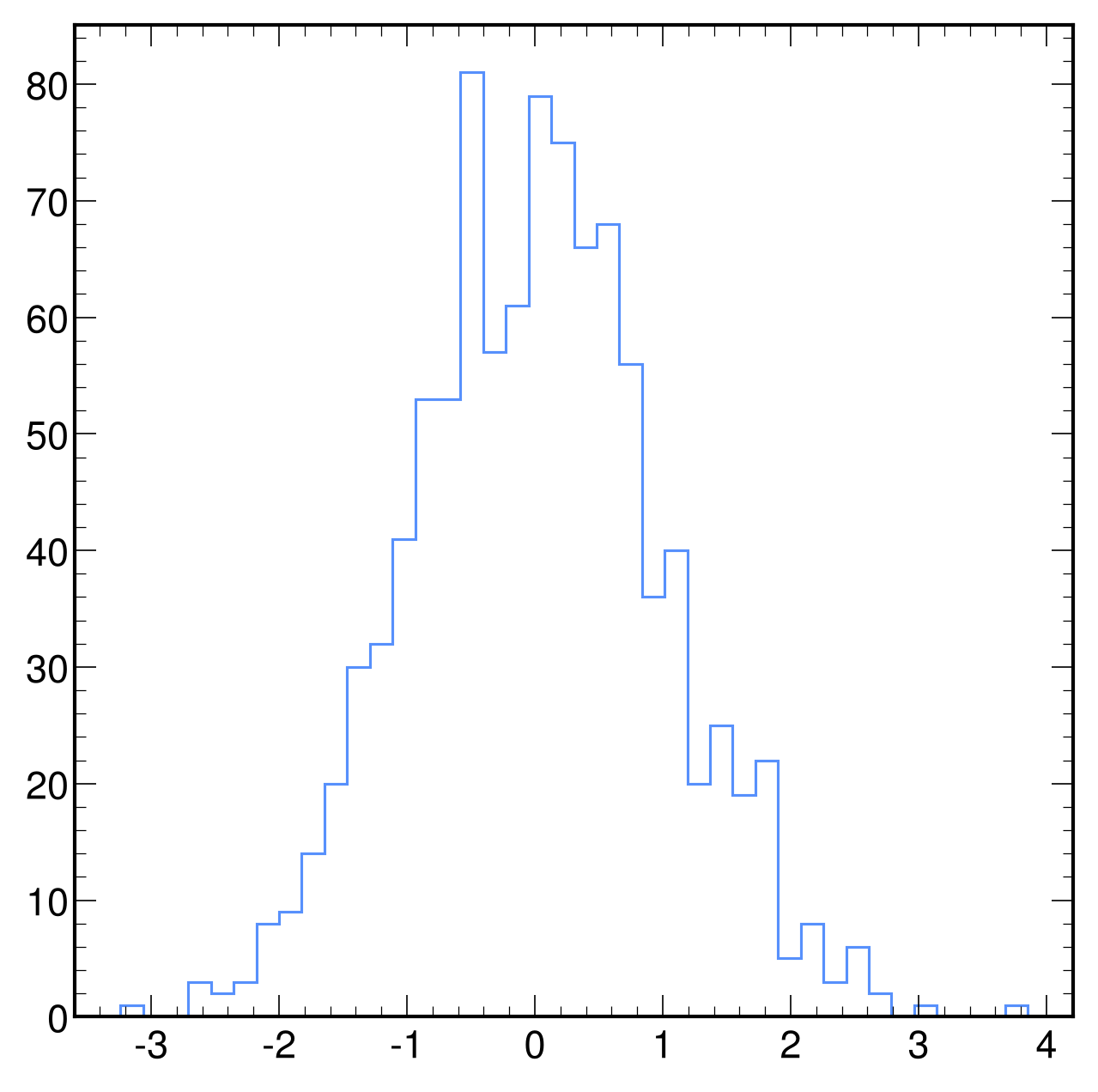
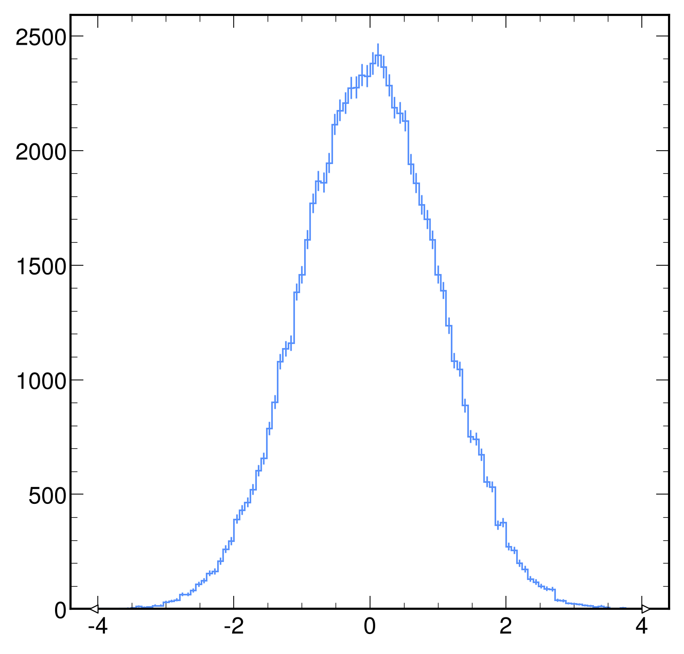
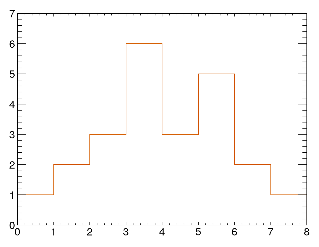
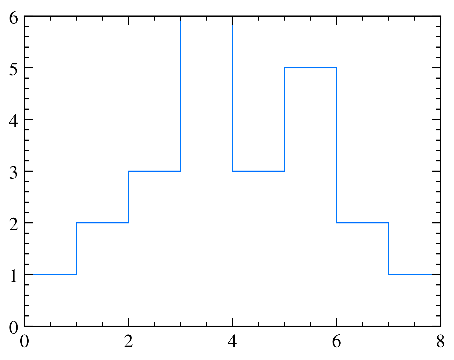
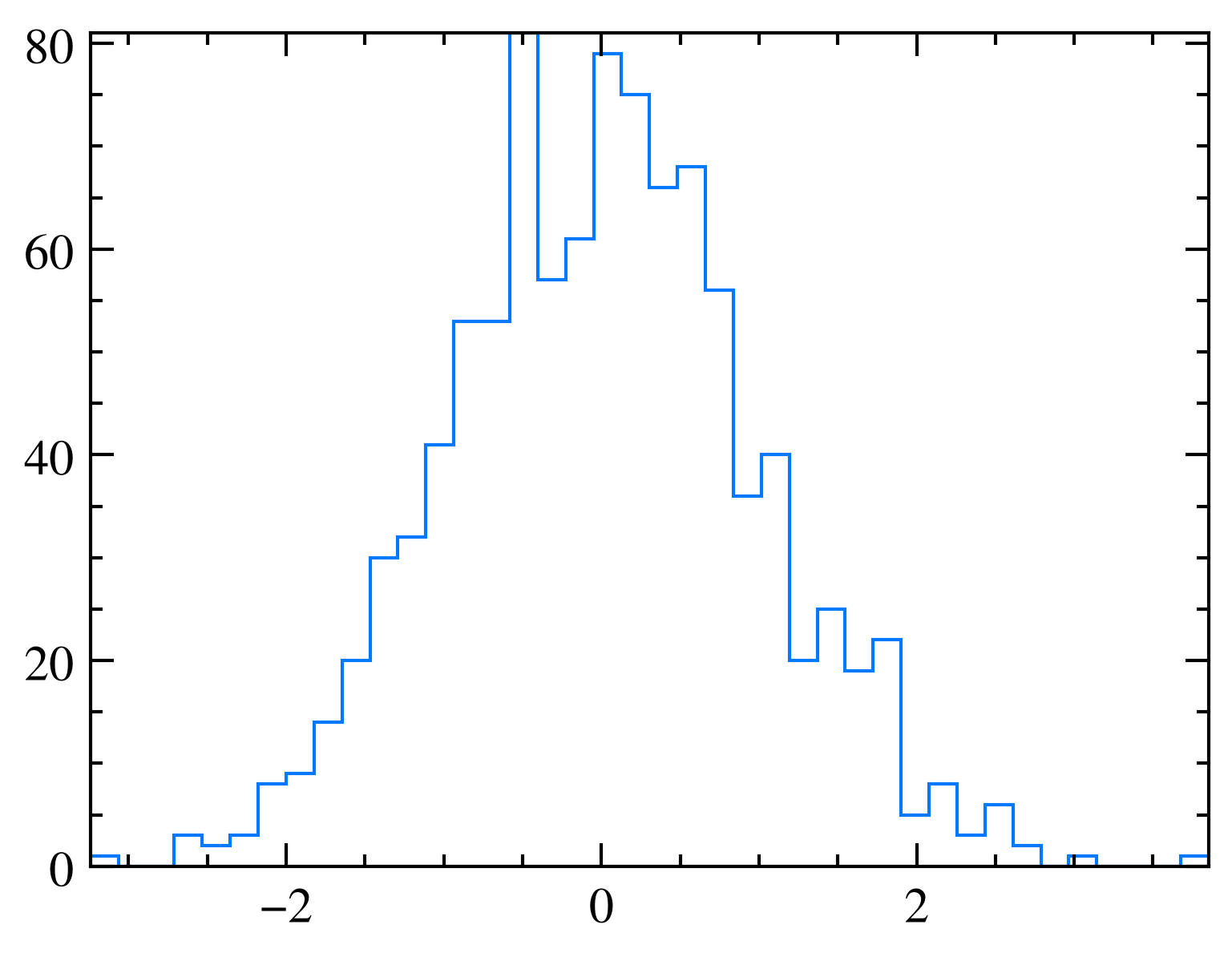
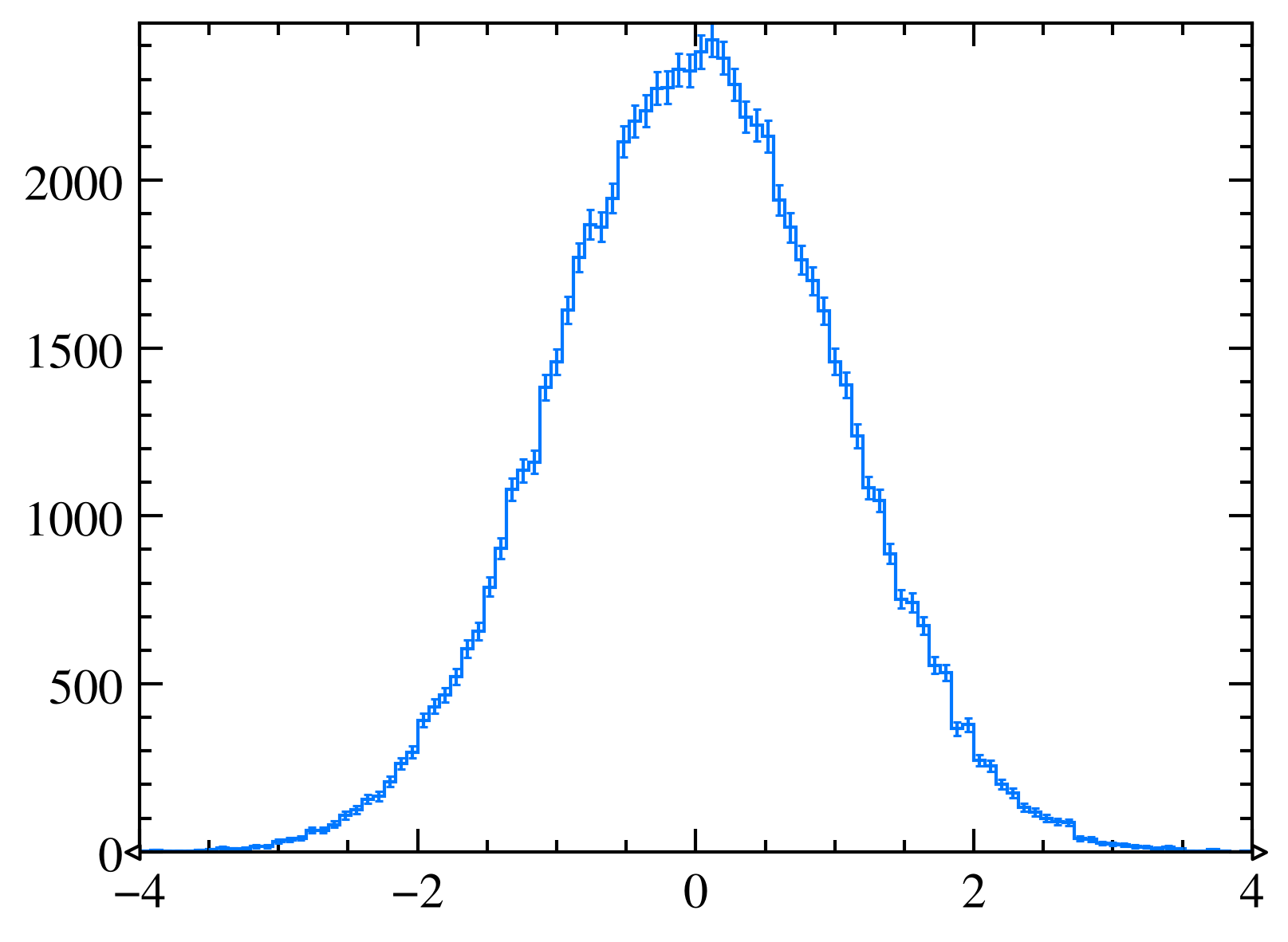
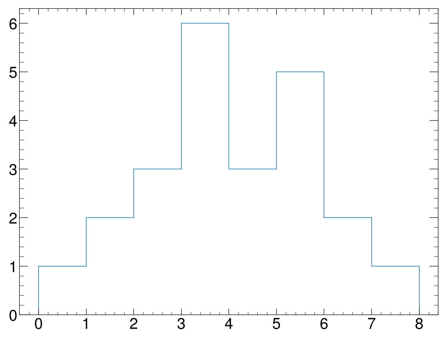
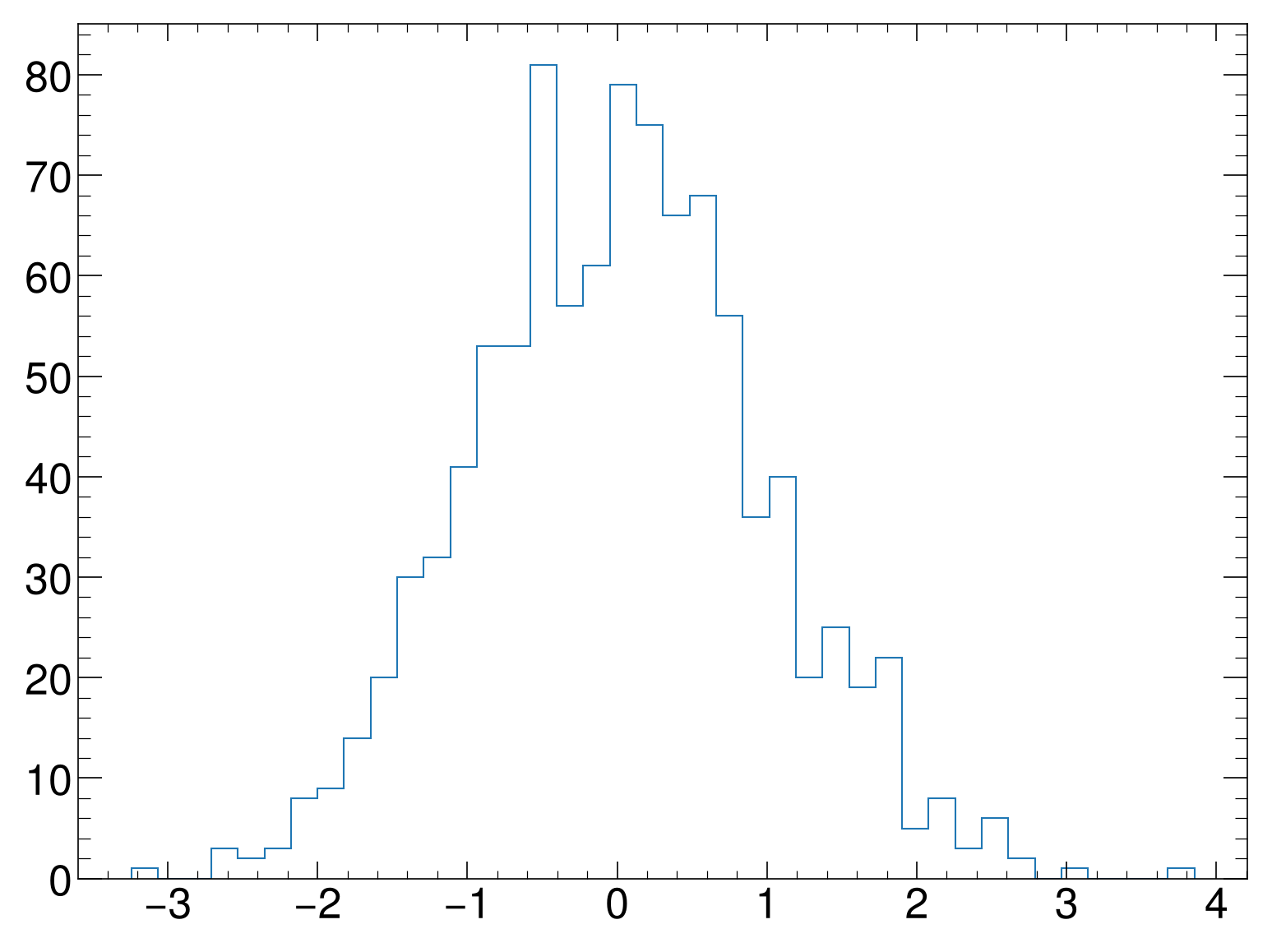
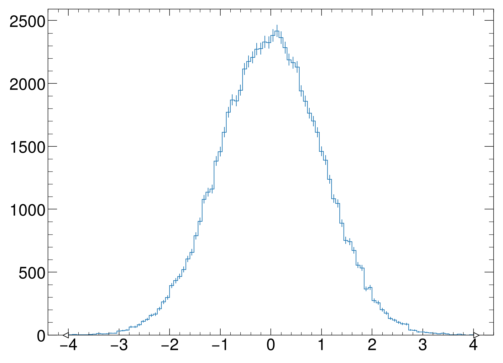
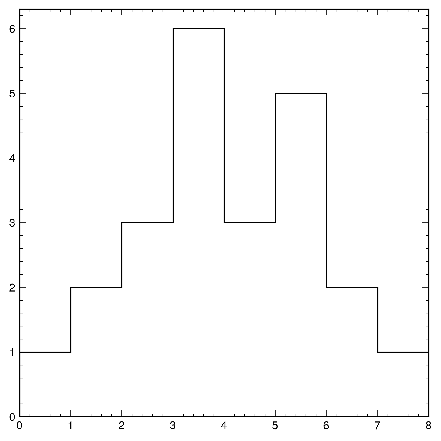
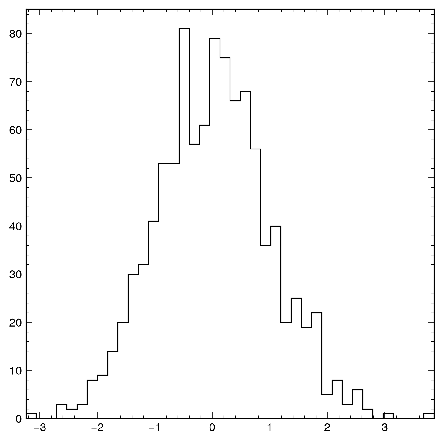
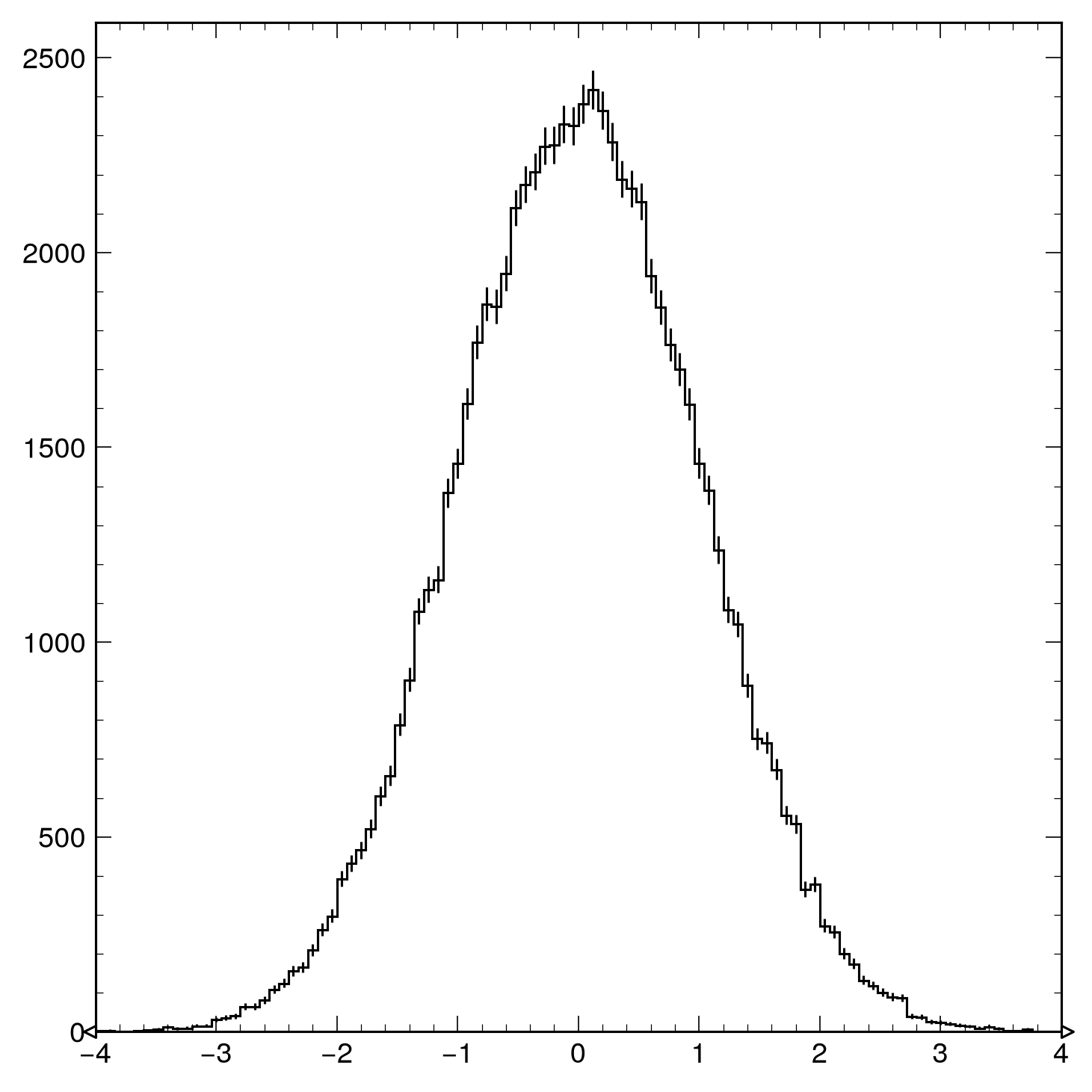
mh.histplot() works with multiple histogram formats through the UHI protocol:
Supported Input Formats¤
Histogram Styles¤
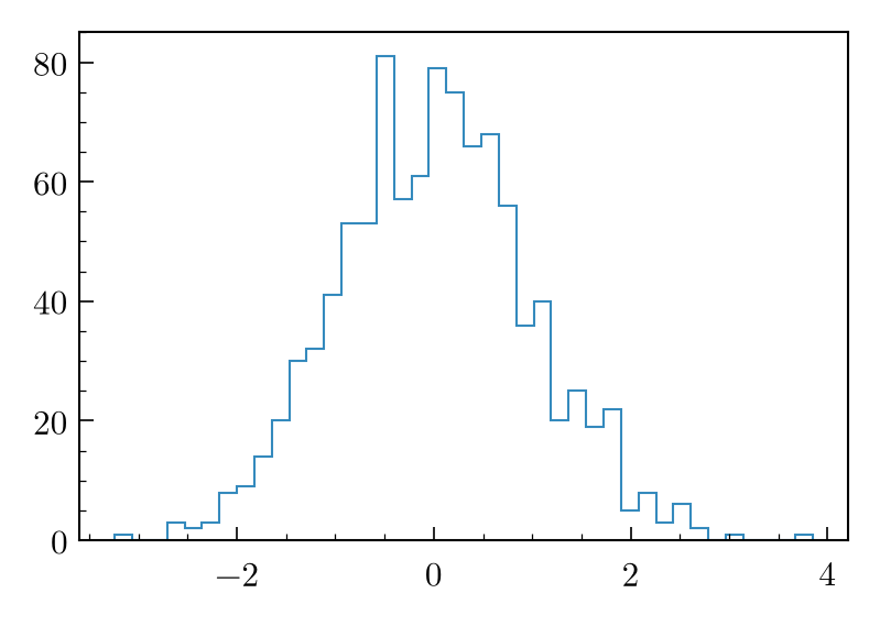
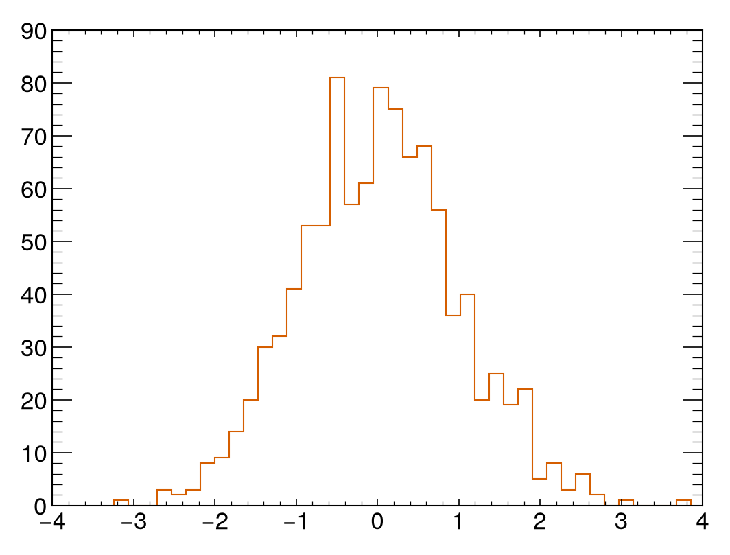
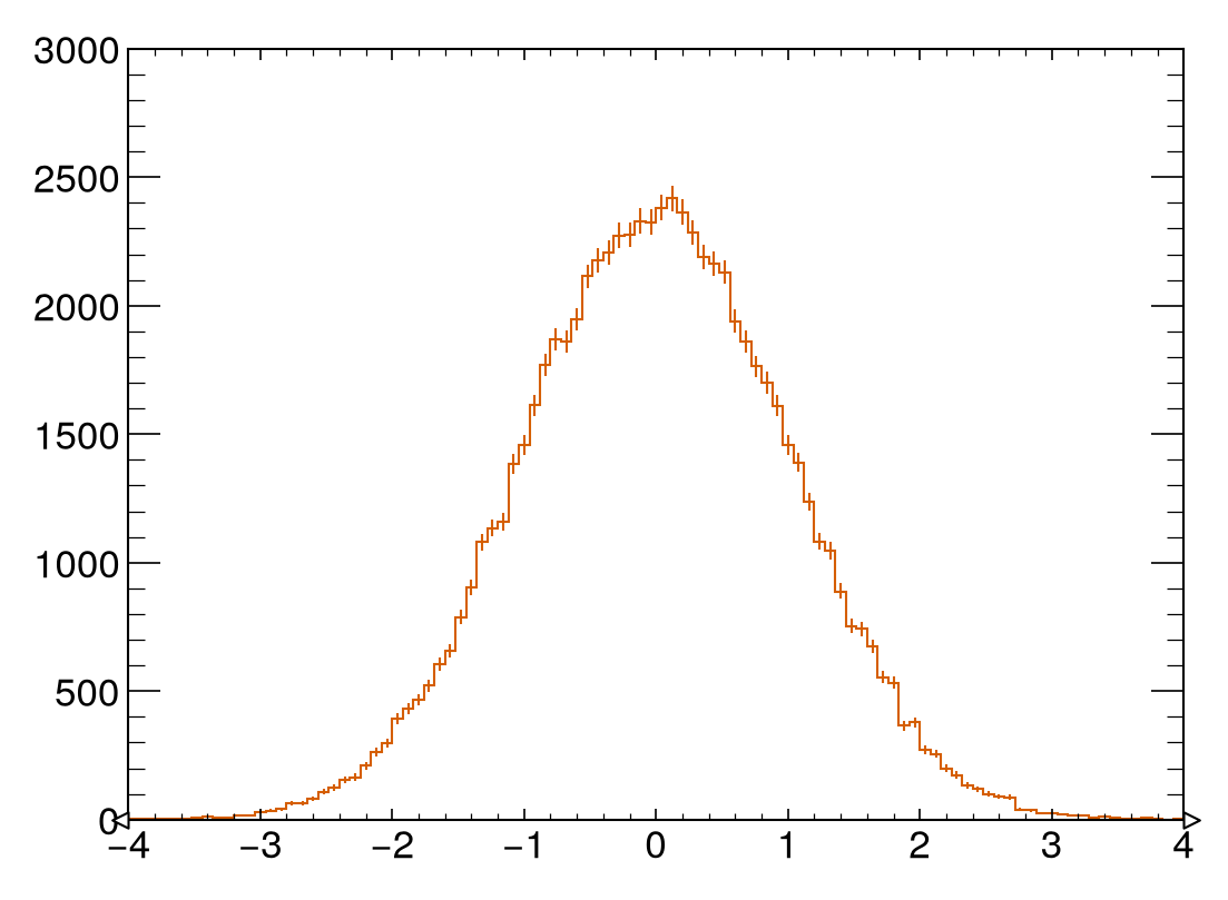
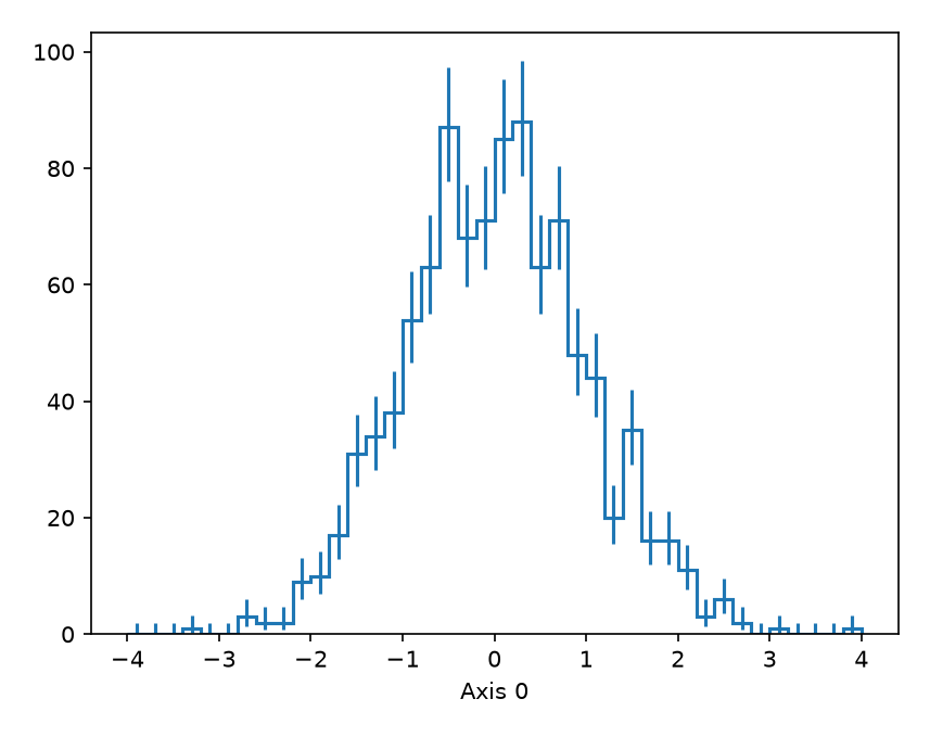
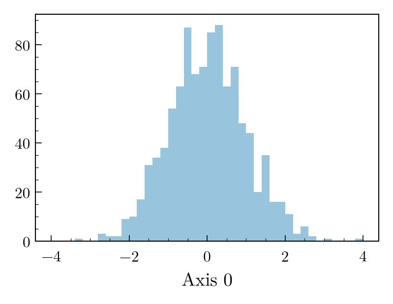
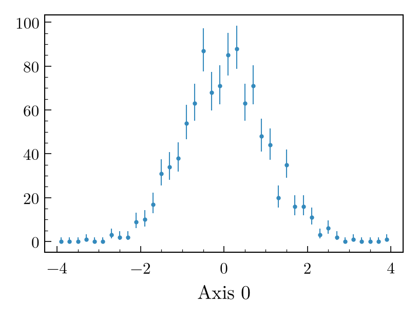
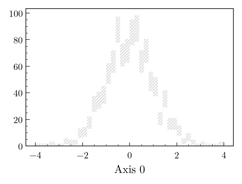
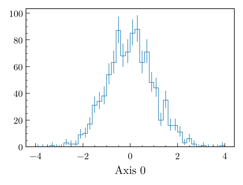
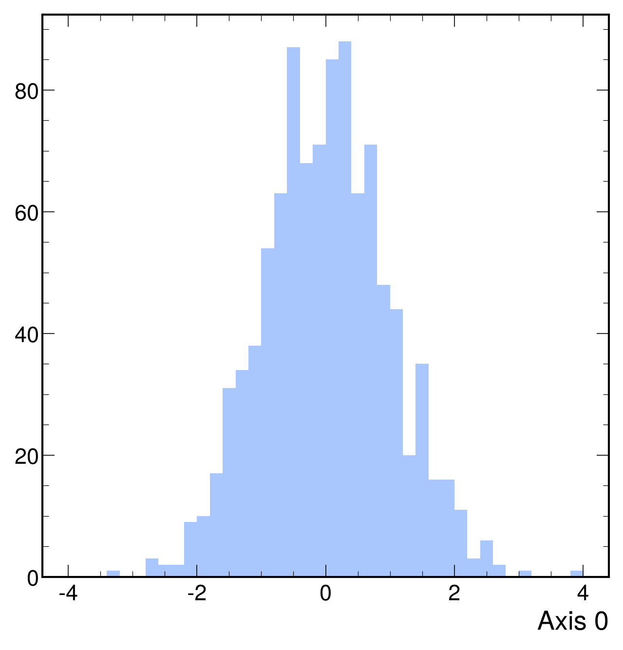
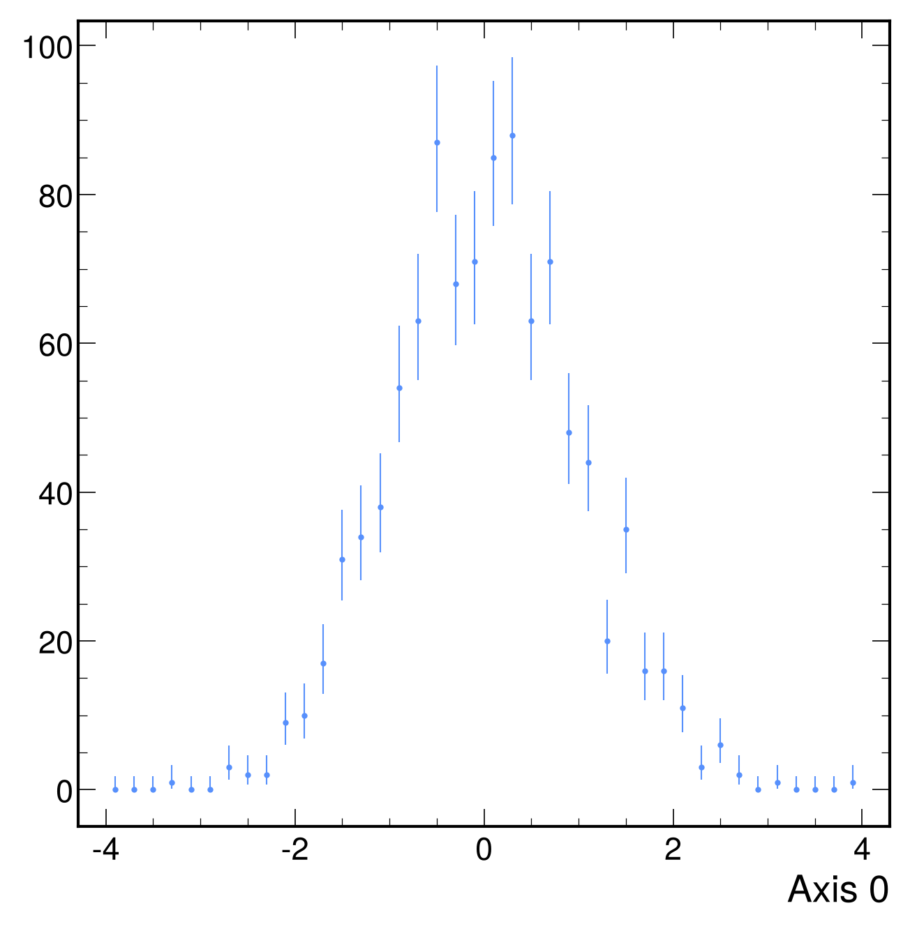
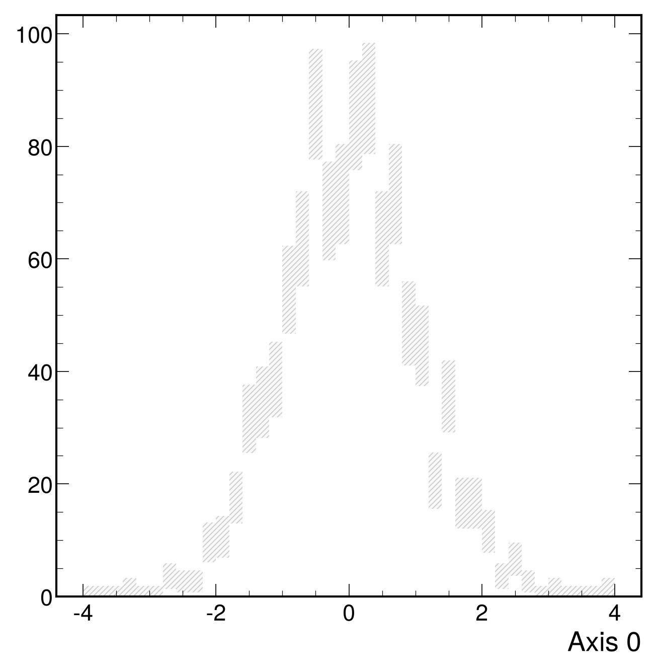
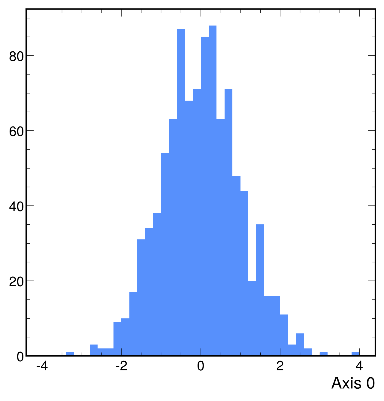
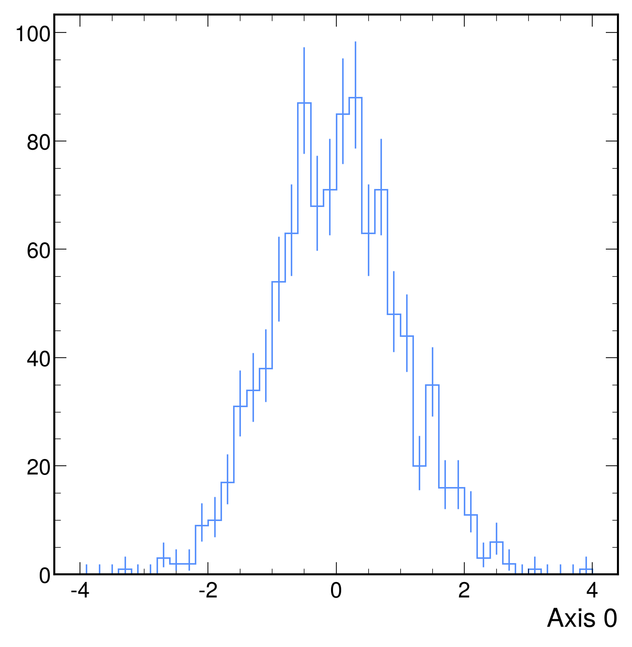
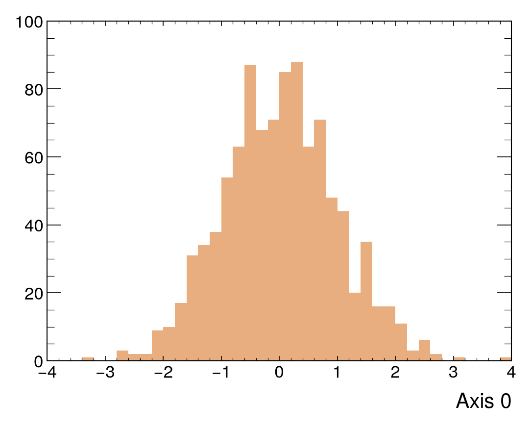
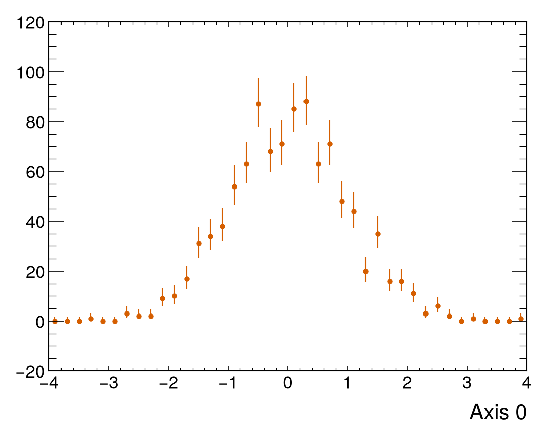
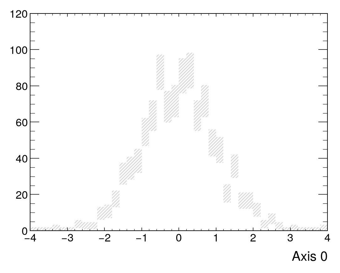
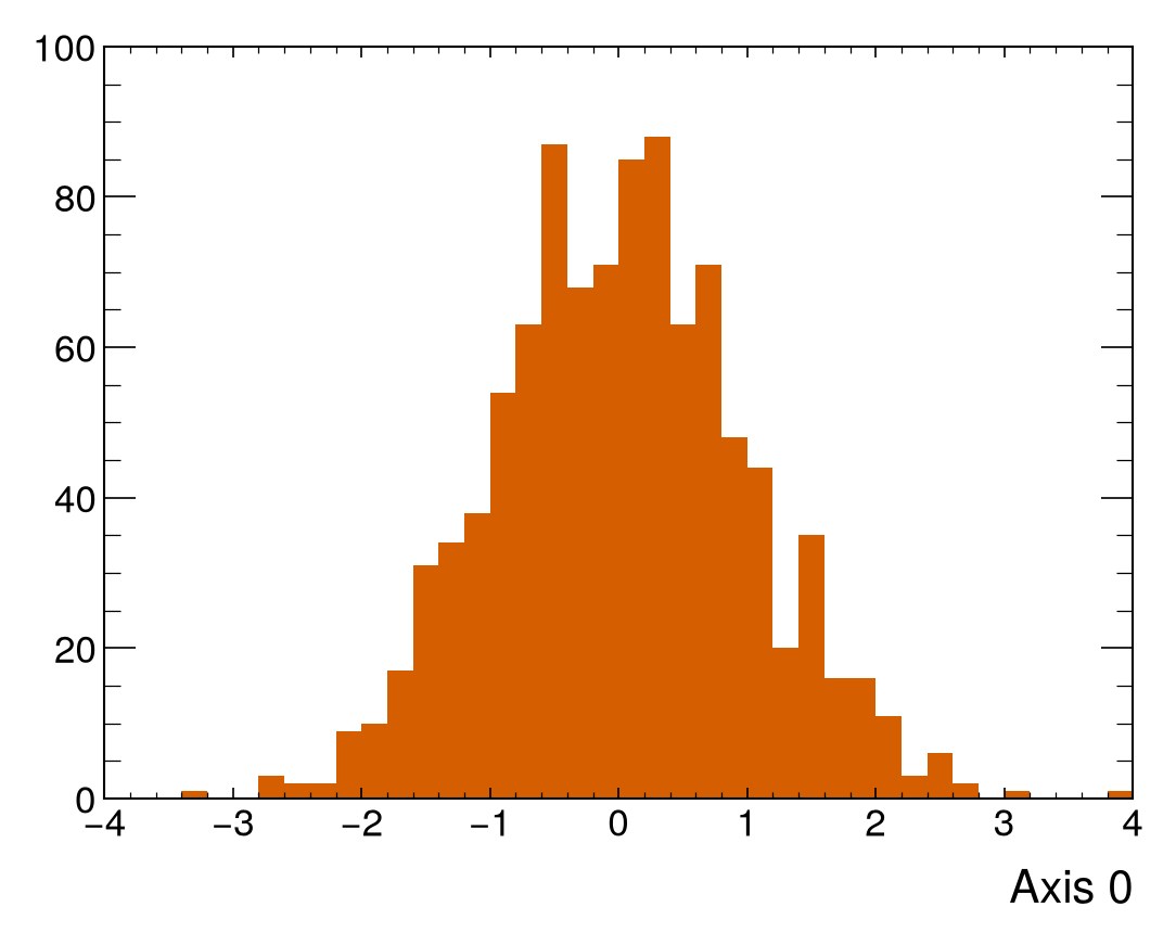
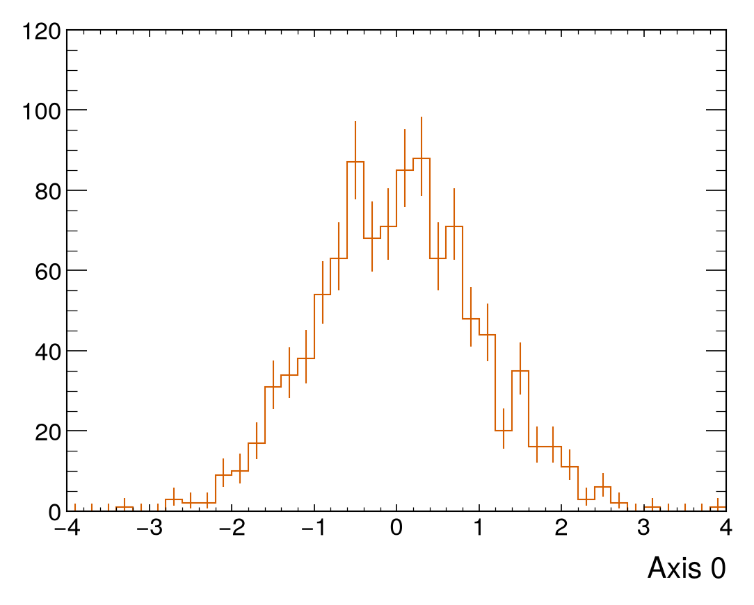
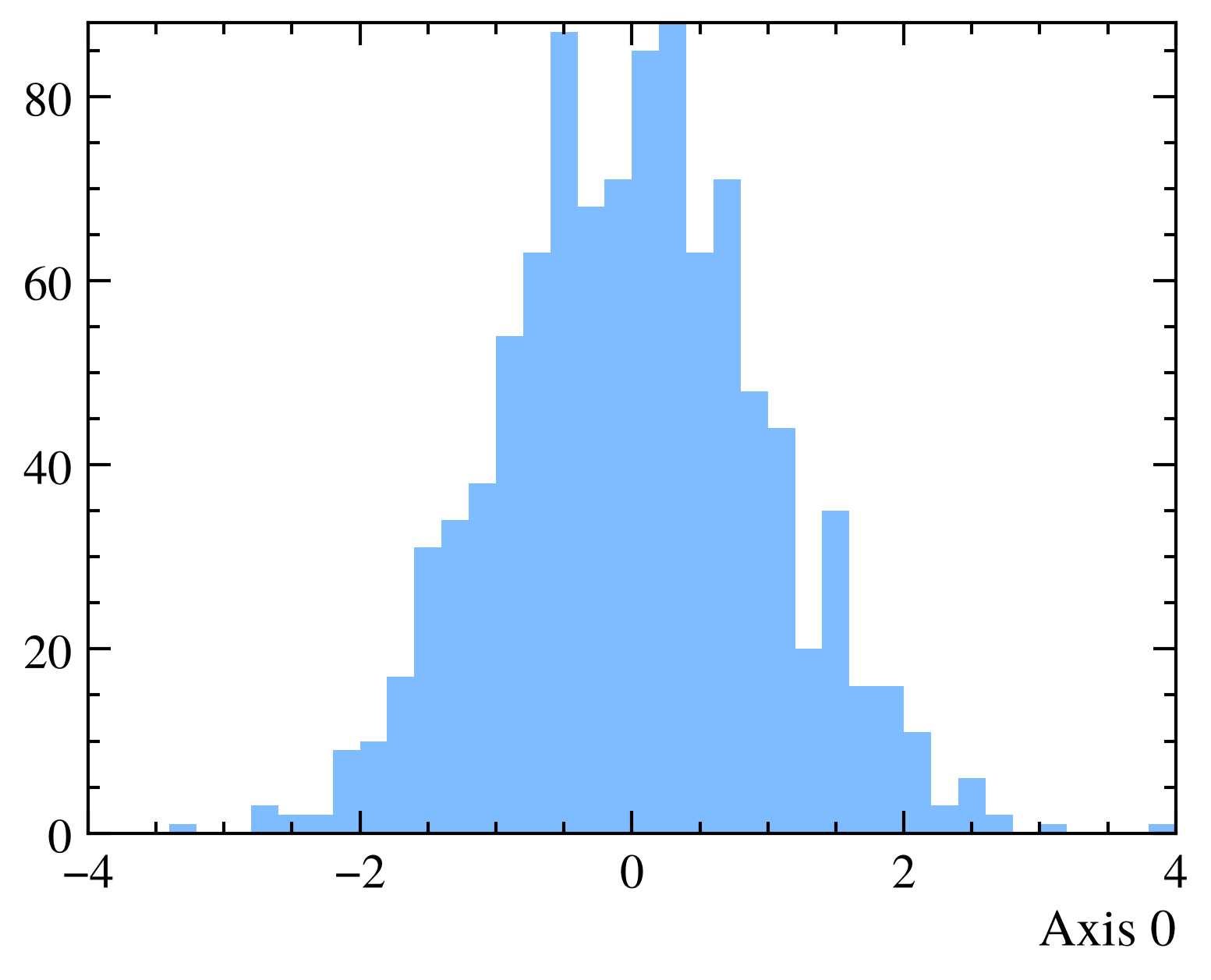
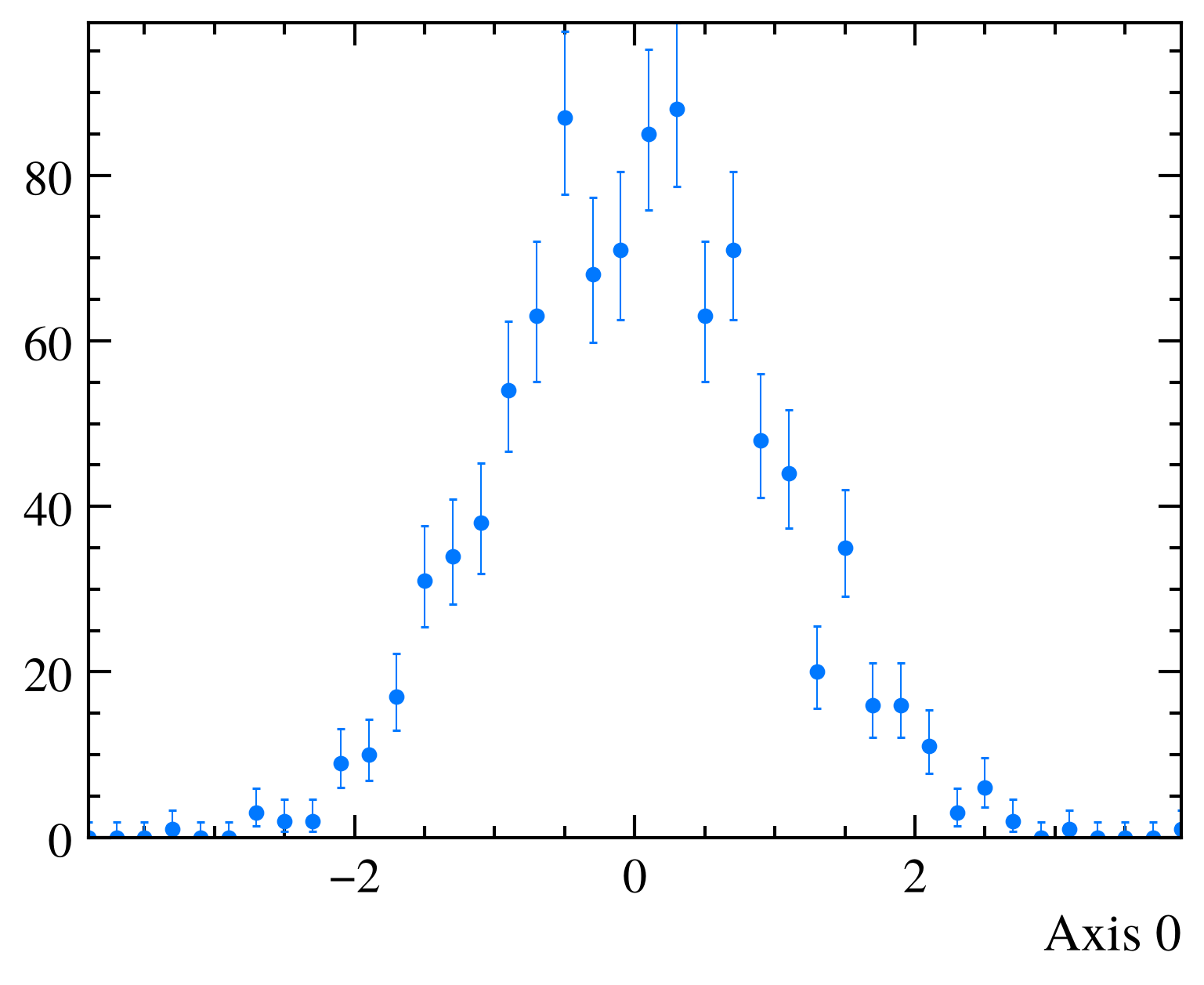
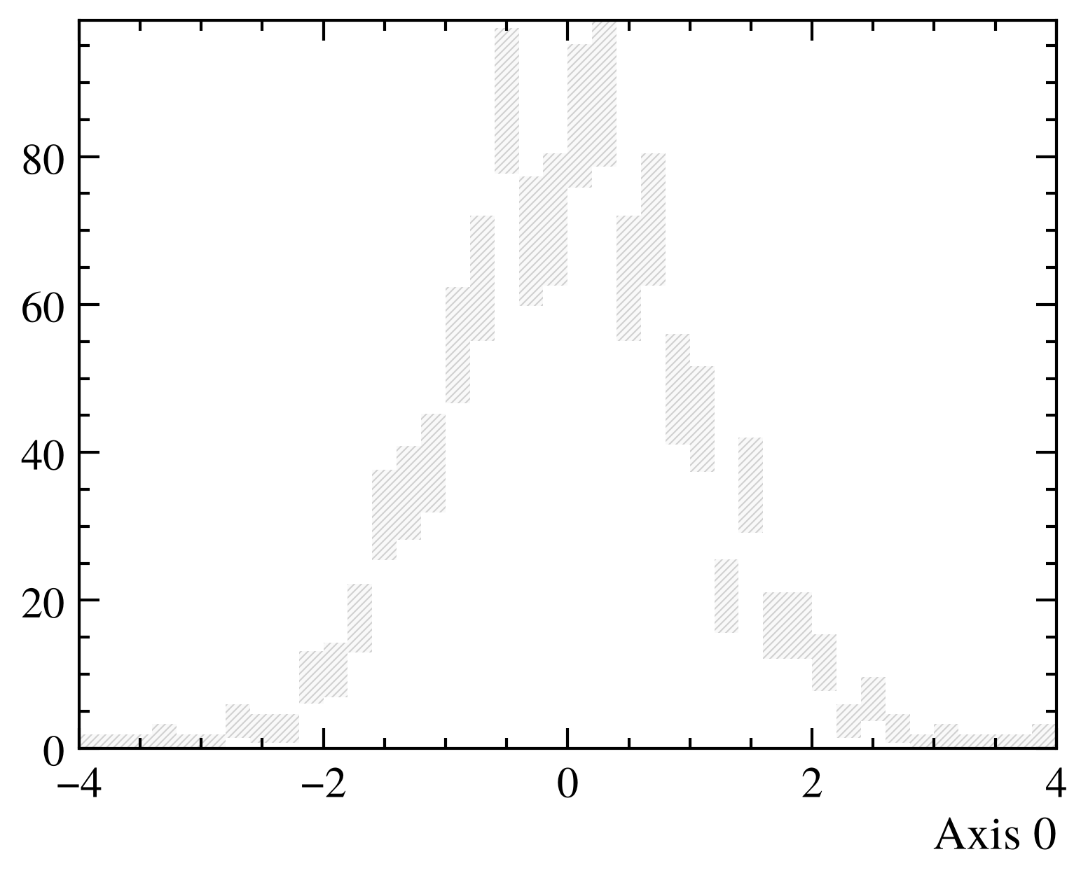
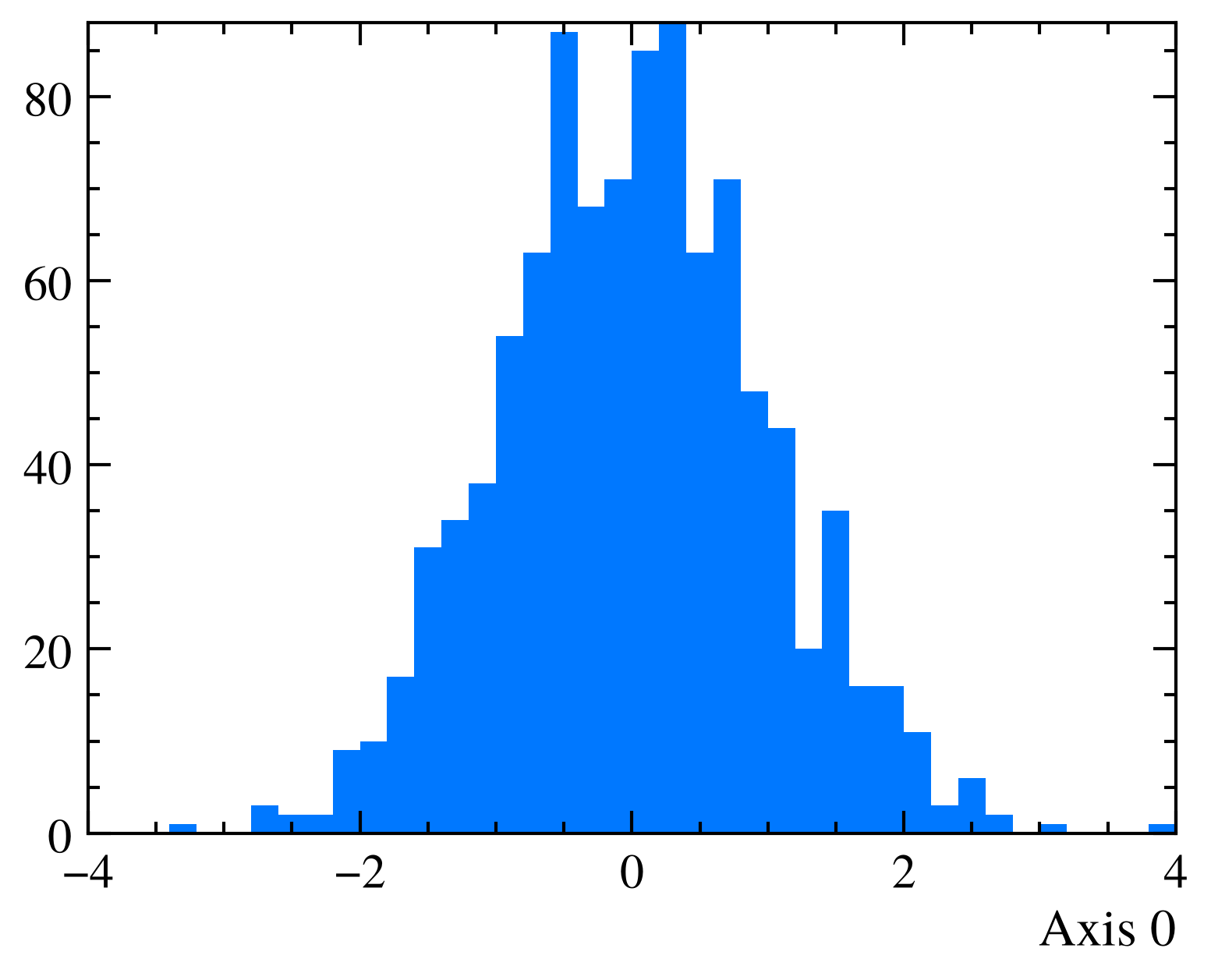
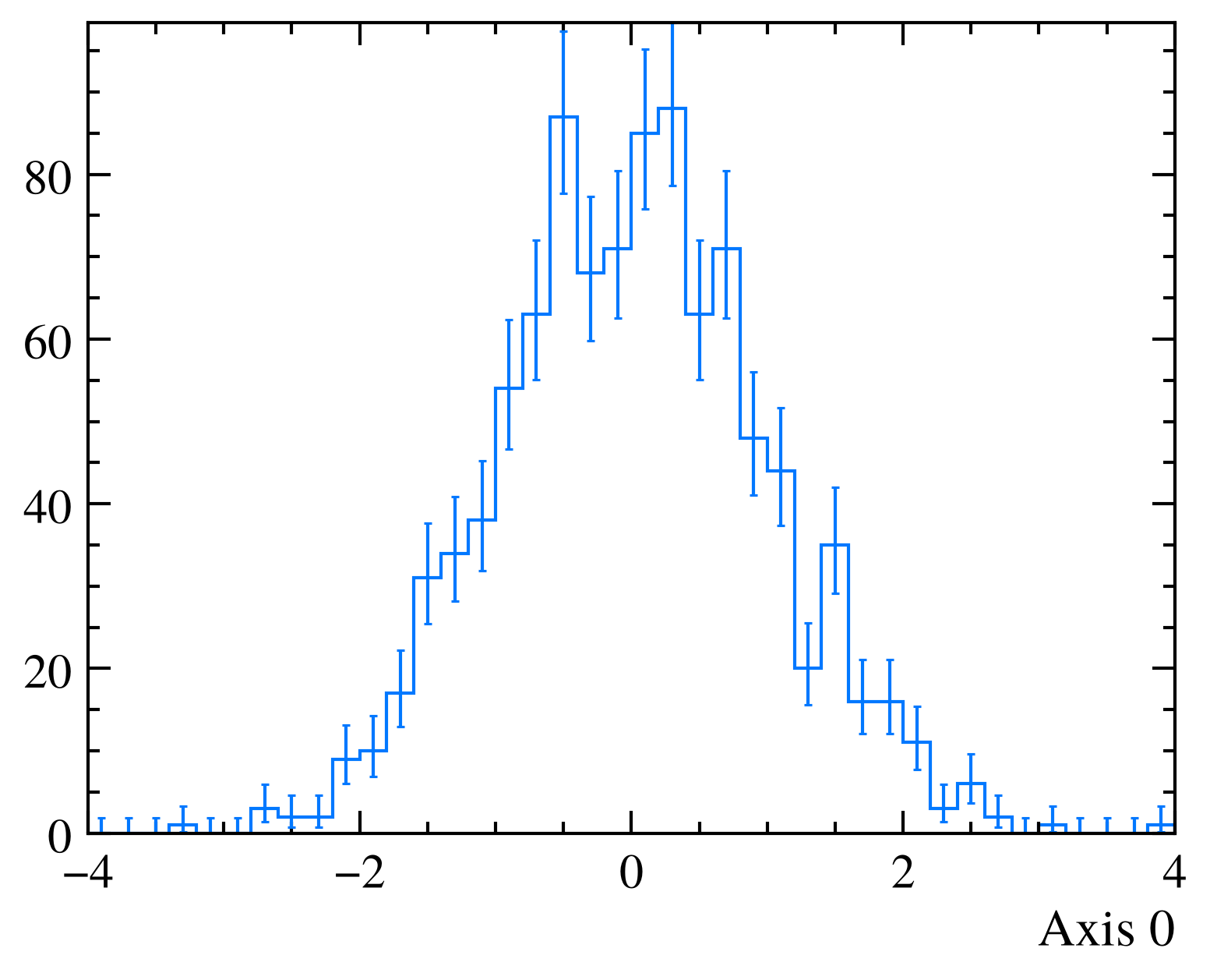
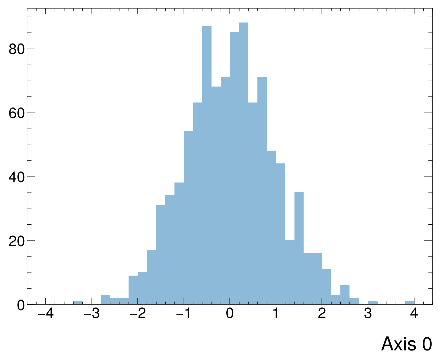
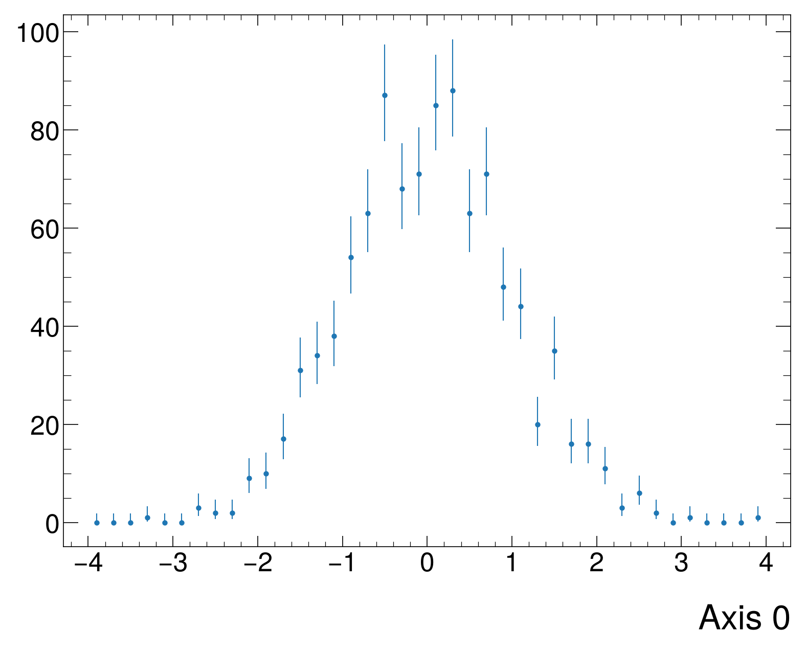
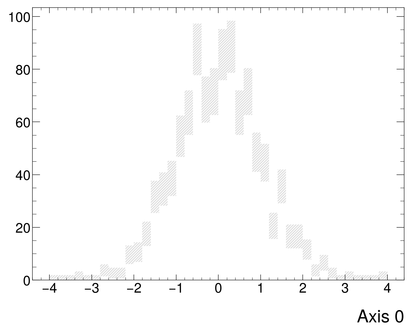
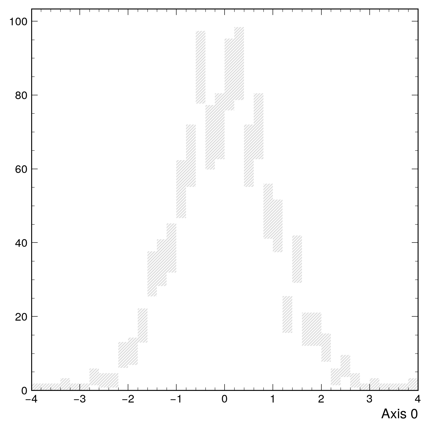
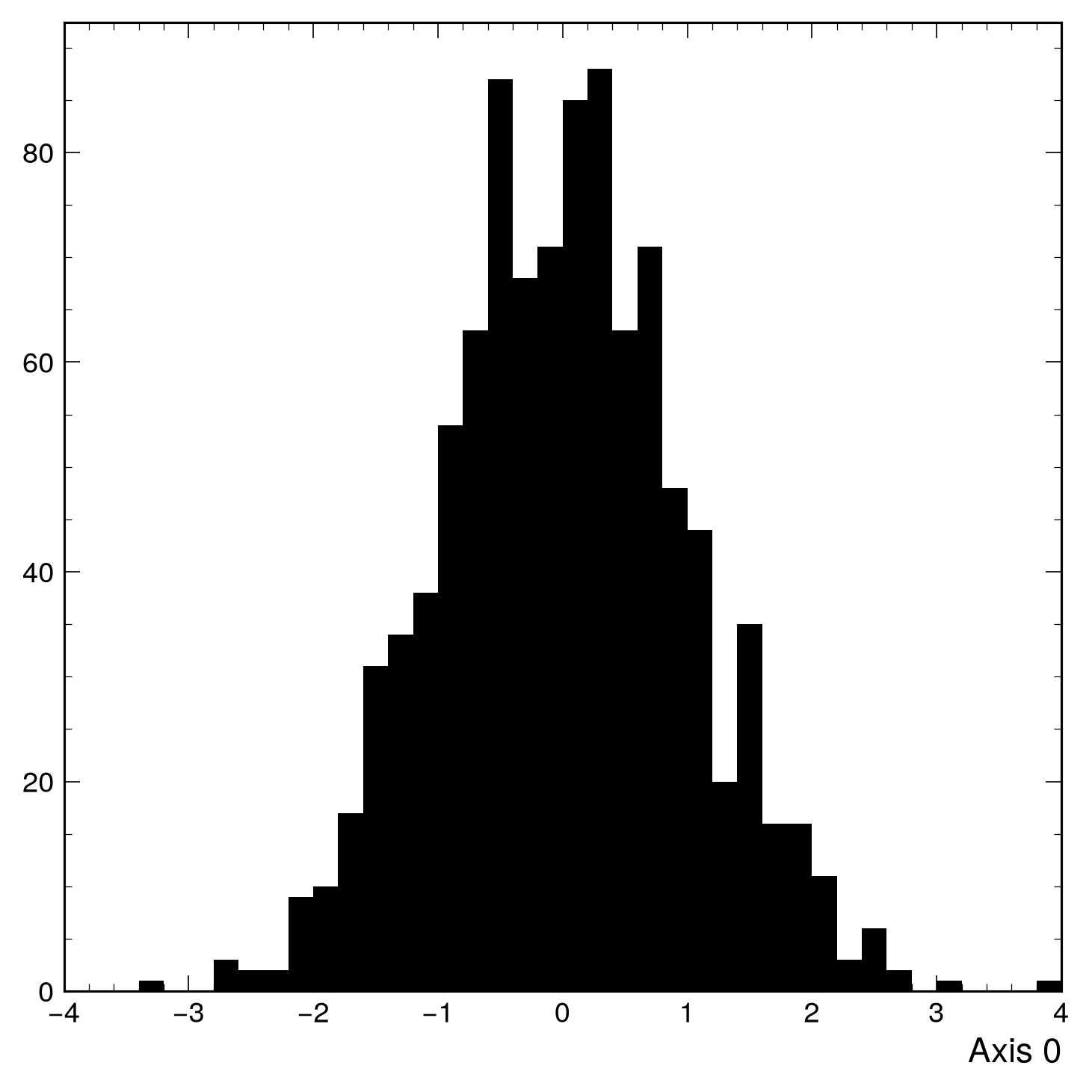
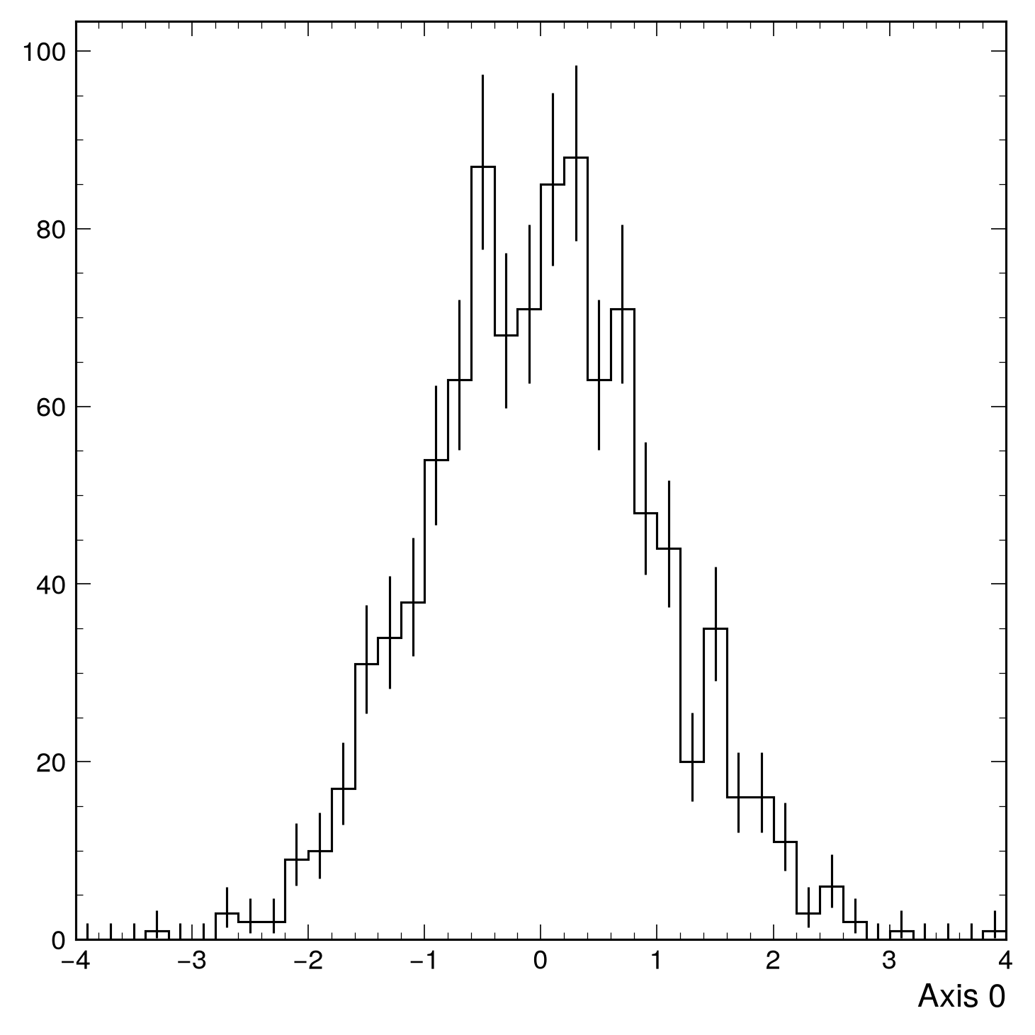
Control the appearance with the histtype parameter. Select an experiment style and then choose a histogram type:
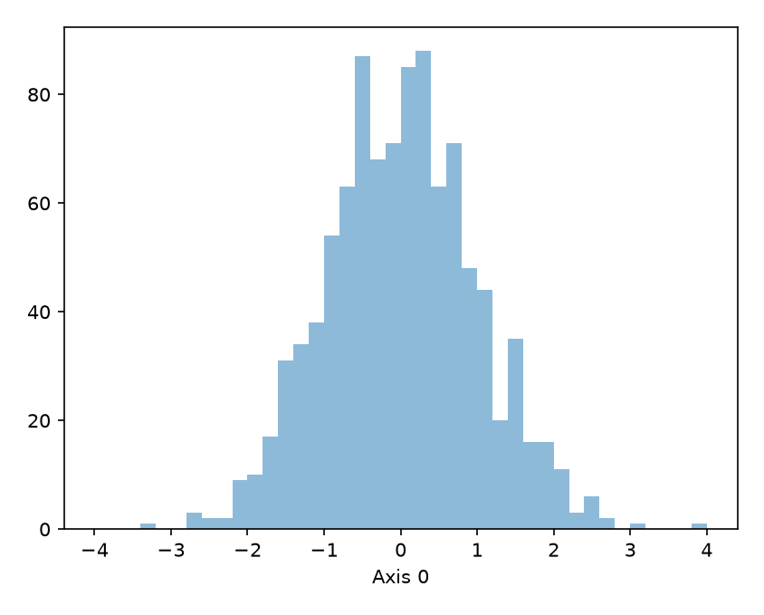
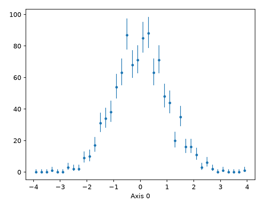
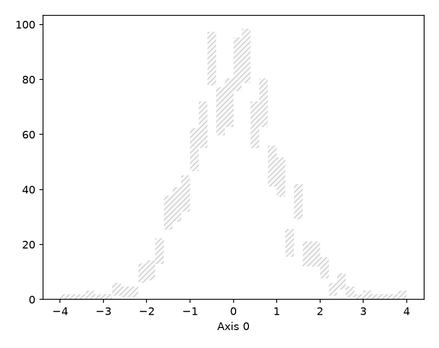
h = hist.new.Reg(40, -4, 4).Weight().fill(np.random.normal(0, 1, 1000))
fig, ax = plt.subplots()
mh.histplot(h, histtype='bar', label='Bar histogram', ax=ax)
# If only one histogram is provided, it will be treated as "fill" histtype, if multiple data are given the bars are arranged side by side (see next section)
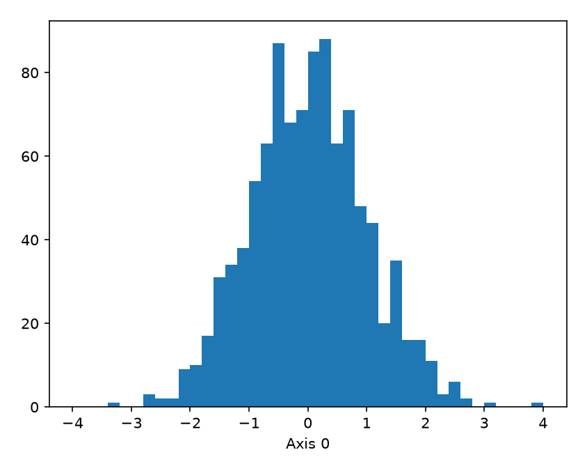
h = hist.new.Reg(40, -4, 4).Weight().fill(np.random.normal(0, 1, 1000))
fig, ax = plt.subplots()
mh.histplot(h, histtype='barstep', label='Barstep histogram', ax=ax)
# If one histogram is provided, it will be treated as "step" histtype. If multiple data are given the bars are arranged side by side (see next section)
h = hist.new.Reg(40, -4, 4).Weight().fill(np.random.normal(0, 1, 1000))
fig, ax = plt.subplots()
mh.histplot(h, histtype='bar', label='Bar histogram', ax=ax)
# If only one histogram is provided, it will be treated as "fill" histtype, if multiple data are given the bars are arranged side by side (see next section)
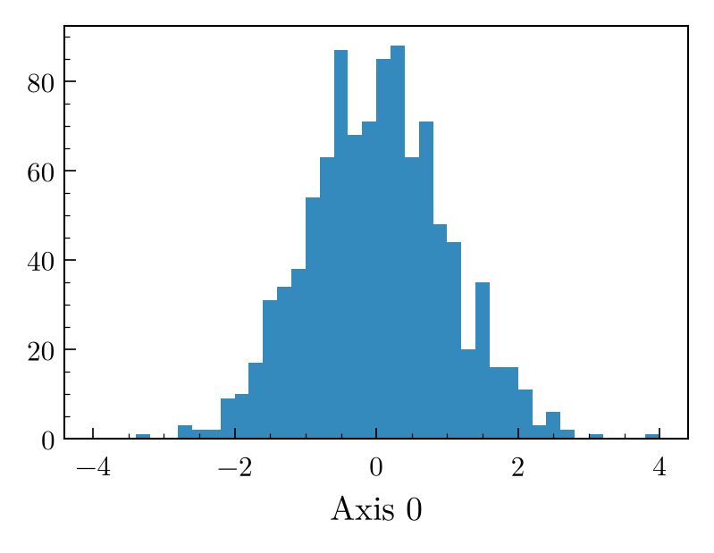
h = hist.new.Reg(40, -4, 4).Weight().fill(np.random.normal(0, 1, 1000))
fig, ax = plt.subplots()
mh.histplot(h, histtype='barstep', label='Barstep histogram', ax=ax)
# If one histogram is provided, it will be treated as "step" histtype. If multiple data are given the bars are arranged side by side (see next section)
h = hist.new.Reg(40, -4, 4).Weight().fill(np.random.normal(0, 1, 1000))
fig, ax = plt.subplots()
mh.histplot(h, histtype='bar', label='Bar histogram', ax=ax)
# If only one histogram is provided, it will be treated as "fill" histtype, if multiple data are given the bars are arranged side by side (see next section)
h = hist.new.Reg(40, -4, 4).Weight().fill(np.random.normal(0, 1, 1000))
fig, ax = plt.subplots()
mh.histplot(h, histtype='barstep', label='Barstep histogram', ax=ax)
# If one histogram is provided, it will be treated as "step" histtype. If multiple data are given the bars are arranged side by side (see next section)
h = hist.new.Reg(40, -4, 4).Weight().fill(np.random.normal(0, 1, 1000))
fig, ax = plt.subplots()
mh.histplot(h, histtype='bar', label='Bar histogram', ax=ax)
# If only one histogram is provided, it will be treated as "fill" histtype, if multiple data are given the bars are arranged side by side (see next section)
h = hist.new.Reg(40, -4, 4).Weight().fill(np.random.normal(0, 1, 1000))
fig, ax = plt.subplots()
mh.histplot(h, histtype='barstep', label='Barstep histogram', ax=ax)
# If one histogram is provided, it will be treated as "step" histtype. If multiple data are given the bars are arranged side by side (see next section)
h = hist.new.Reg(40, -4, 4).Weight().fill(np.random.normal(0, 1, 1000))
fig, ax = plt.subplots()
mh.histplot(h, histtype='bar', label='Bar histogram', ax=ax)
# If only one histogram is provided, it will be treated as "fill" histtype, if multiple data are given the bars are arranged side by side (see next section)
h = hist.new.Reg(40, -4, 4).Weight().fill(np.random.normal(0, 1, 1000))
fig, ax = plt.subplots()
mh.histplot(h, histtype='barstep', label='Barstep histogram', ax=ax)
# If one histogram is provided, it will be treated as "step" histtype. If multiple data are given the bars are arranged side by side (see next section)
h = hist.new.Reg(40, -4, 4).Weight().fill(np.random.normal(0, 1, 1000))
fig, ax = plt.subplots()
mh.histplot(h, histtype='bar', label='Bar histogram', ax=ax)
# If only one histogram is provided, it will be treated as "fill" histtype, if multiple data are given the bars are arranged side by side (see next section)
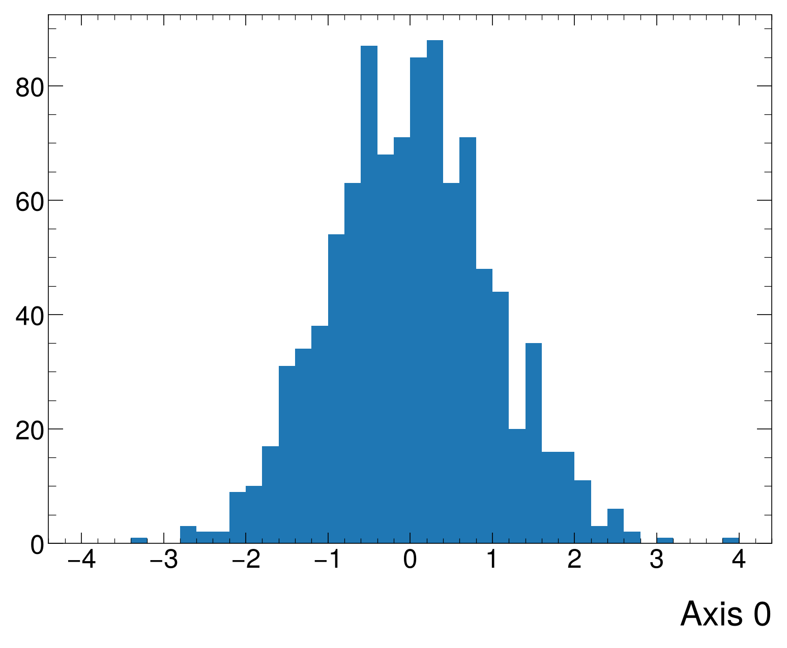
h = hist.new.Reg(40, -4, 4).Weight().fill(np.random.normal(0, 1, 1000))
fig, ax = plt.subplots()
mh.histplot(h, histtype='barstep', label='Barstep histogram', ax=ax)
# If one histogram is provided, it will be treated as "step" histtype. If multiple data are given the bars are arranged side by side (see next section)
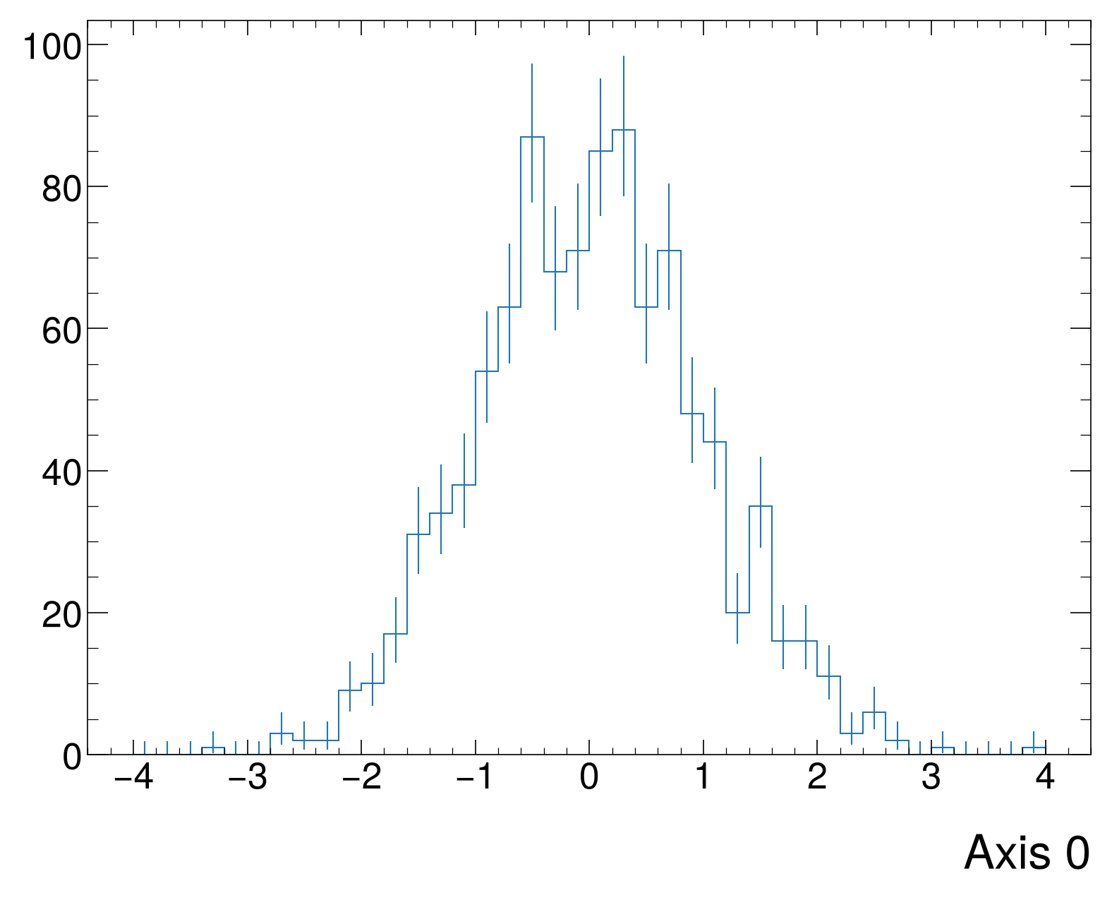
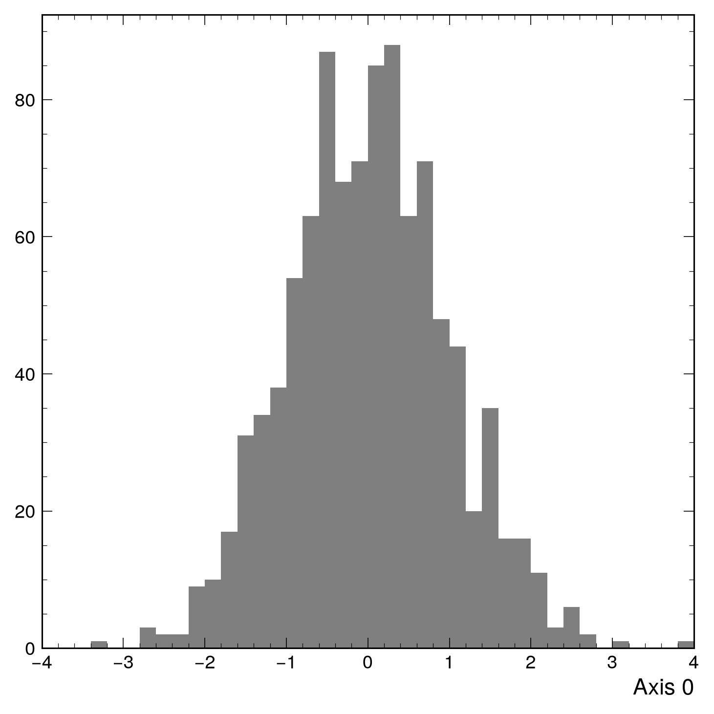
h = hist.new.Reg(40, -4, 4).Weight().fill(np.random.normal(0, 1, 1000))
fig, ax = plt.subplots()
mh.histplot(h, histtype='bar', label='Bar histogram', ax=ax)
# If only one histogram is provided, it will be treated as "fill" histtype, if multiple data are given the bars are arranged side by side (see next section)
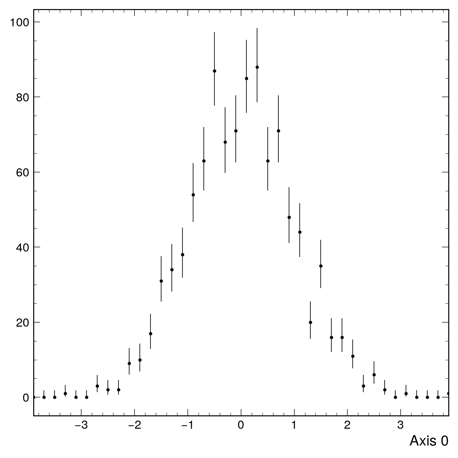
h = hist.new.Reg(40, -4, 4).Weight().fill(np.random.normal(0, 1, 1000))
fig, ax = plt.subplots()
mh.histplot(h, histtype='barstep', label='Barstep histogram', ax=ax)
# If one histogram is provided, it will be treated as "step" histtype. If multiple data are given the bars are arranged side by side (see next section)
Multiple Histograms¤
Stack¤
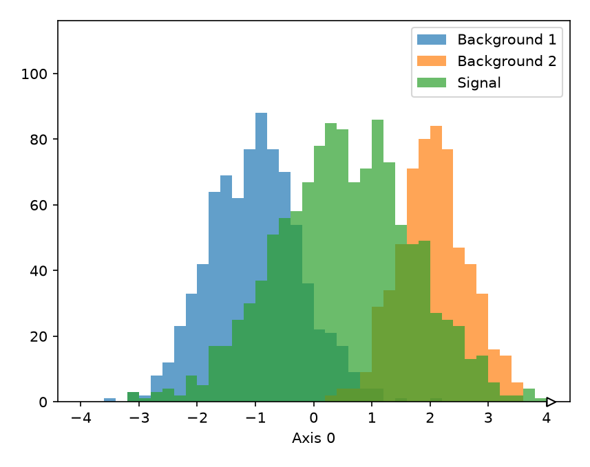
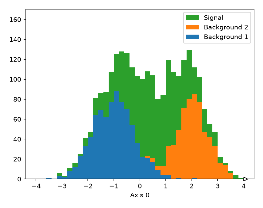
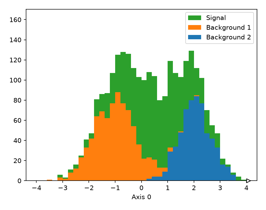
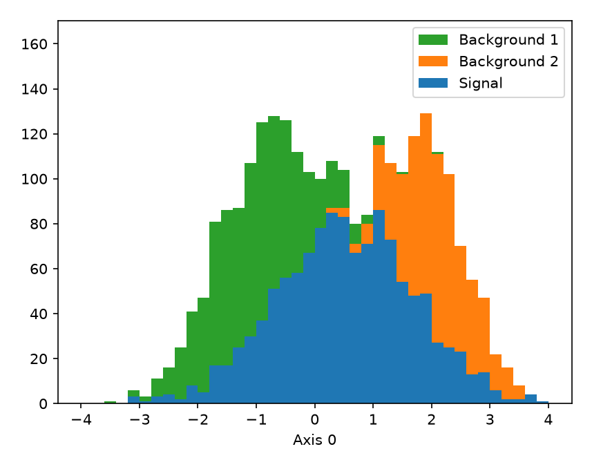
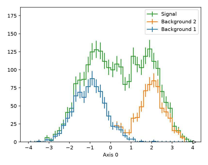
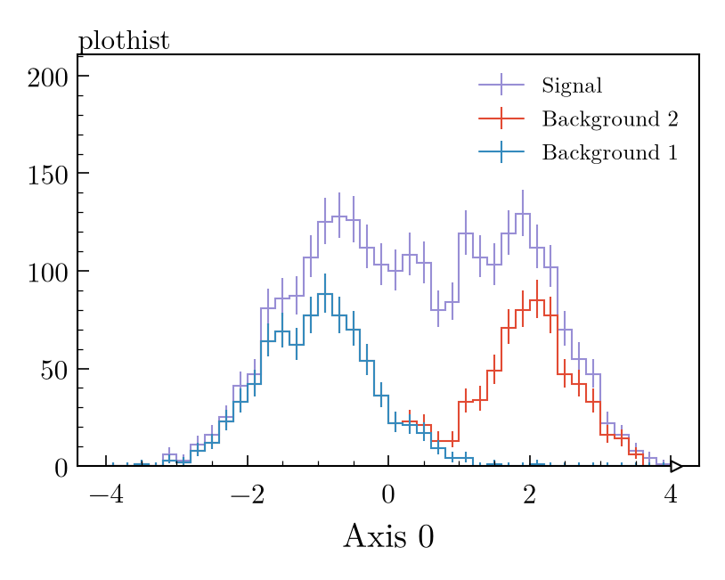
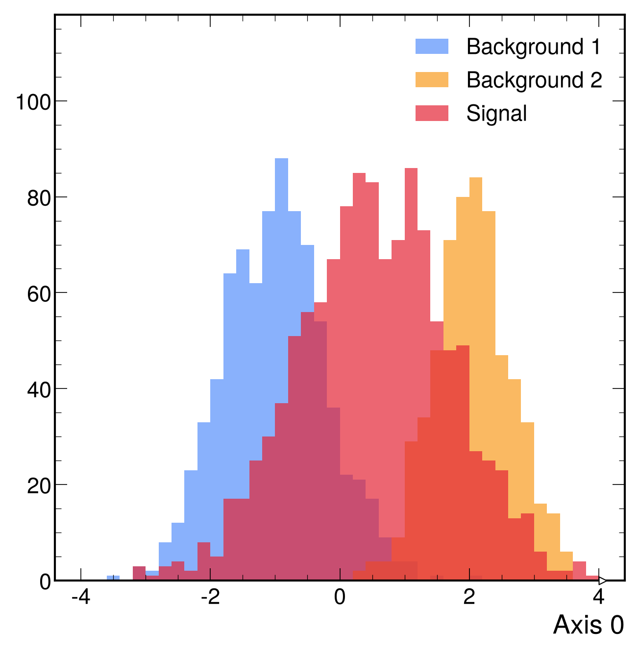
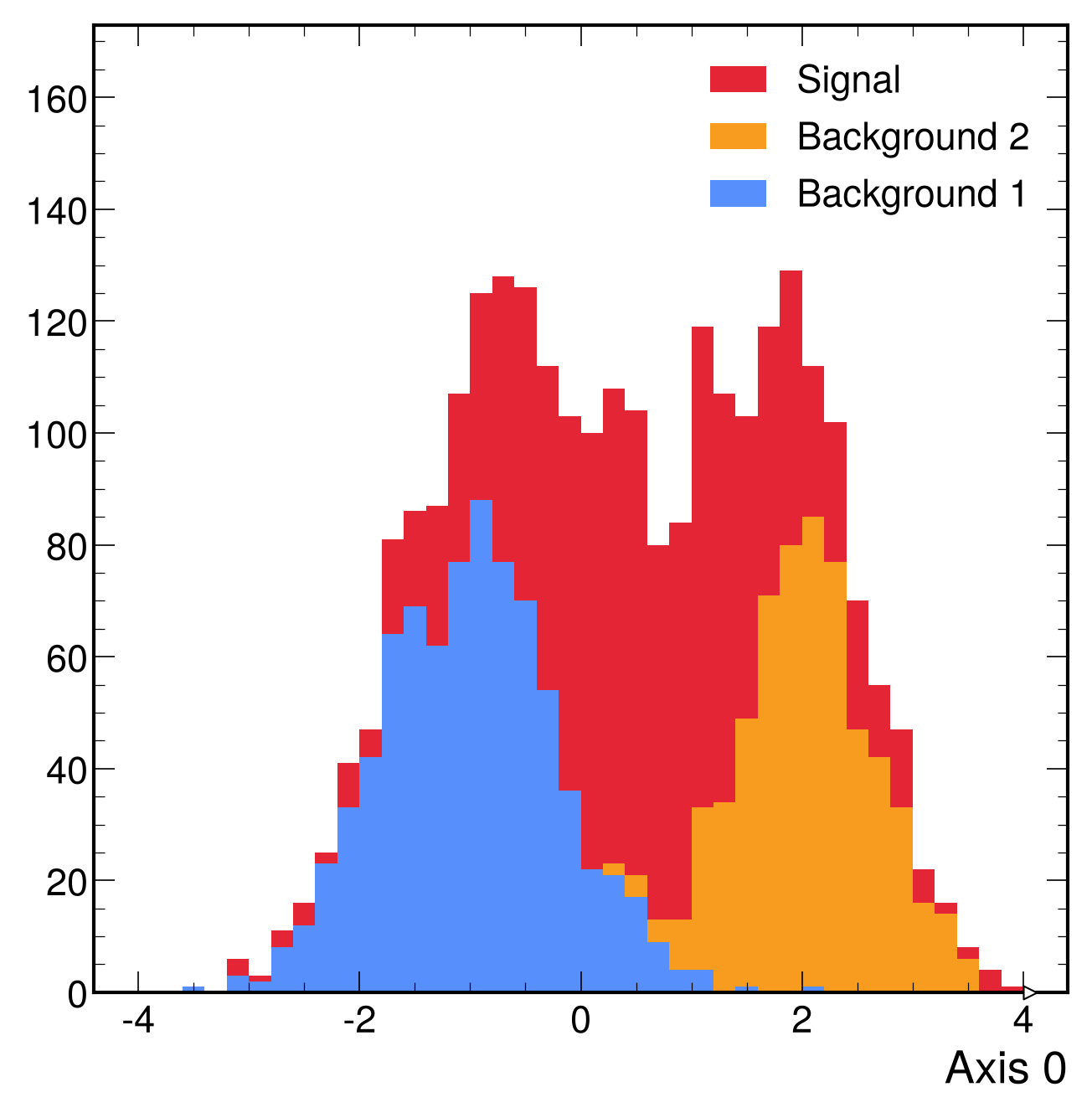
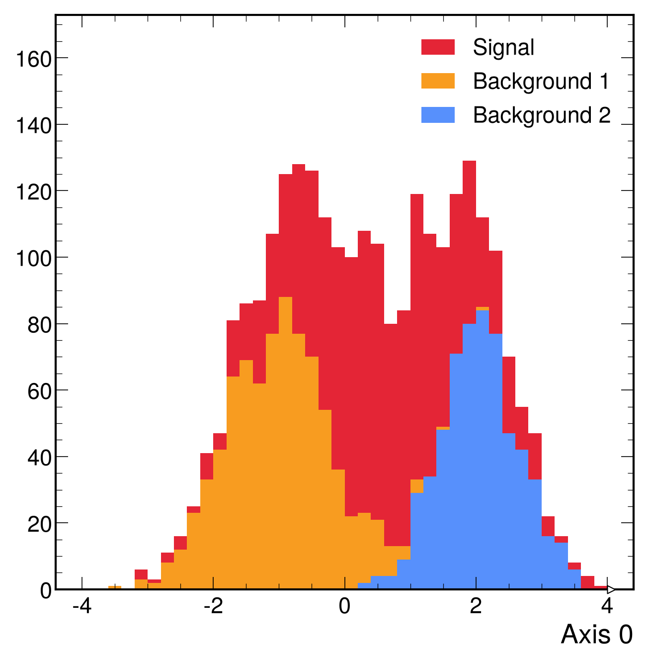
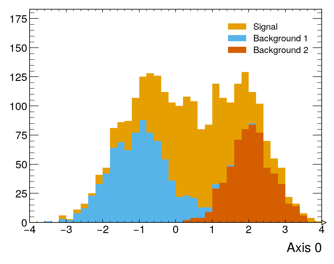
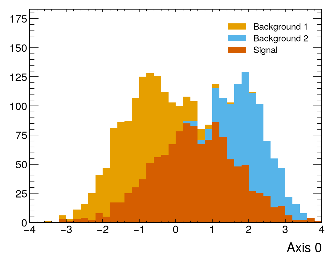
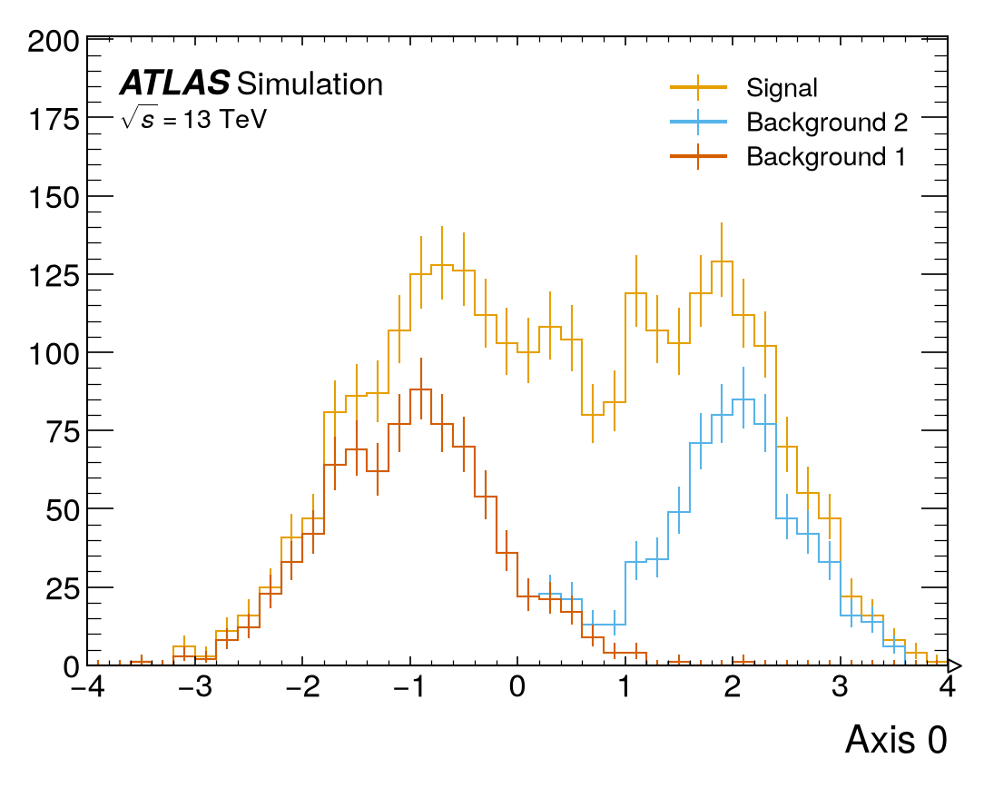
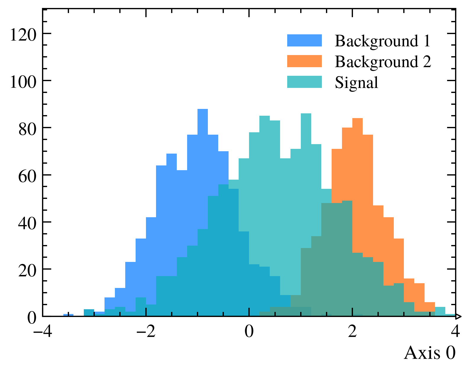
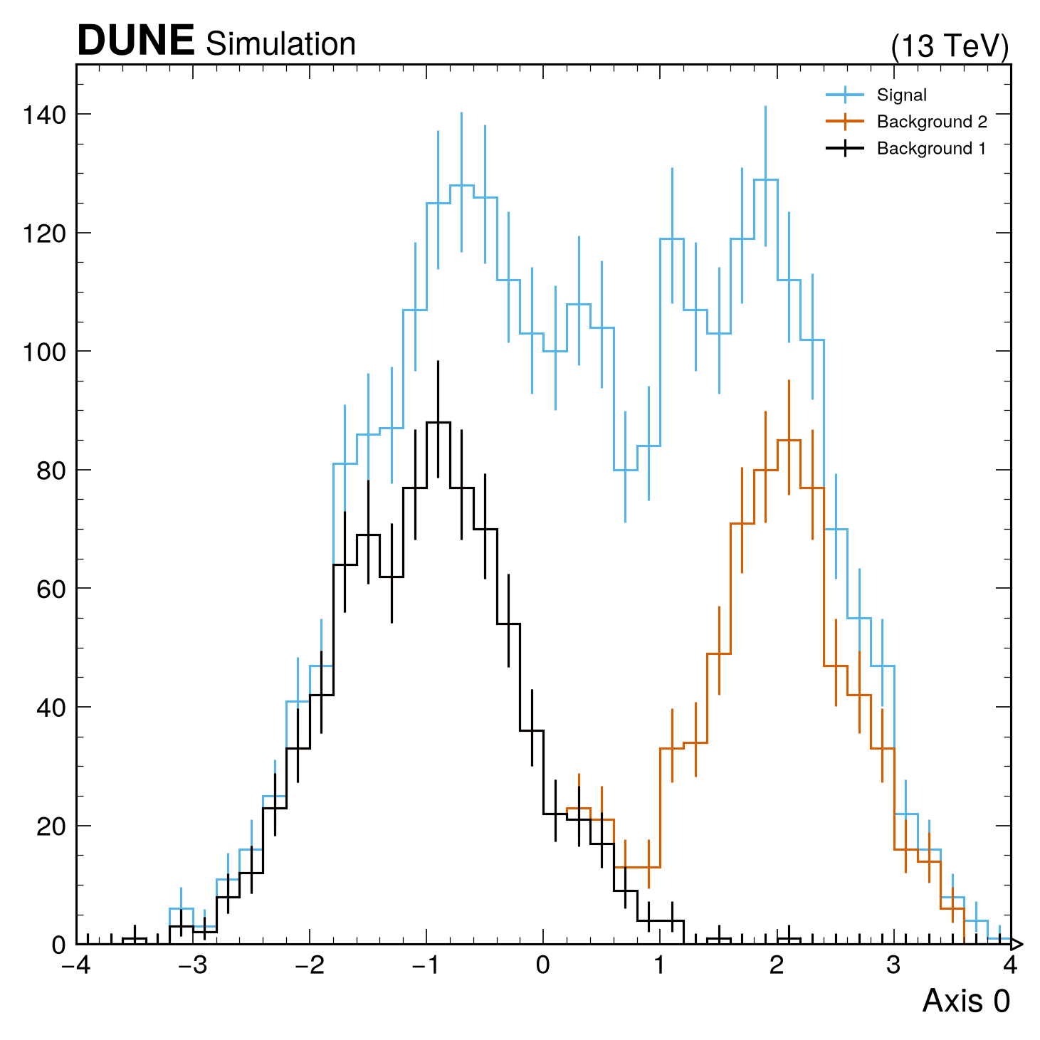
mh.histplot() supports plotting multiple histograms in one call. They can be stacked using the stack=True parameter:
# Create histograms and fill them
h1 = hist.new.Reg(40, -4, 4).Weight().fill(np.random.normal(-1, 0.8, 800))
h2 = hist.new.Reg(40, -4, 4).Weight().fill(np.random.normal(2, 0.6, 600))
h3 = hist.new.Reg(40, -4, 4).Weight().fill(np.random.normal(0.5, 1.2, 1200))

fig, ax = plt.subplots()
mh.histplot(
 [h1, h2, h3],
 histtype='fill',
 alpha=0.7,
 label=['Background 1', 'Background 2', 'Signal'],
 ax=ax
)
ax.legend(loc='upper right')
mh.yscale_legend(soft_fail=True)
# Create histograms and fill them
h1 = hist.new.Reg(40, -4, 4).Weight().fill(np.random.normal(-1, 0.8, 800))
h2 = hist.new.Reg(40, -4, 4).Weight().fill(np.random.normal(2, 0.6, 600))
h3 = hist.new.Reg(40, -4, 4).Weight().fill(np.random.normal(0.5, 1.2, 1200))

fig, ax = plt.subplots()
mh.histplot(
 [h1, h2, h3],
 histtype='fill',
 stack=True,
 label=['Background 1', 'Background 2', 'Signal'],
 ax=ax
)
ax.legend(loc='upper right')
mh.yscale_legend(soft_fail=True)
# Create histograms and fill them
h1 = hist.new.Reg(40, -4, 4).Weight().fill(np.random.normal(-1, 0.8, 800))
h2 = hist.new.Reg(40, -4, 4).Weight().fill(np.random.normal(2, 0.6, 600))
h3 = hist.new.Reg(40, -4, 4).Weight().fill(np.random.normal(0.5, 1.2, 1200))

fig, ax = plt.subplots()
mh.histplot(
 [h1, h2, h3],
 histtype='fill',
 stack=True,
 sort='yield',
 label=['Background 1', 'Background 2', 'Signal'],
 ax=ax
)
ax.legend(loc='upper right')
mh.yscale_legend(soft_fail=True)
# Create histograms and fill them
h1 = hist.new.Reg(40, -4, 4).Weight().fill(np.random.normal(-1, 0.8, 800))
h2 = hist.new.Reg(40, -4, 4).Weight().fill(np.random.normal(2, 0.6, 600))
h3 = hist.new.Reg(40, -4, 4).Weight().fill(np.random.normal(0.5, 1.2, 1200))

fig, ax = plt.subplots()
mh.histplot(
 [h1, h2, h3],
 histtype='fill',
 stack=True,
 sort='label',
 label=['Background 1', 'Background 2', 'Signal'],
 ax=ax
)
ax.legend(loc='upper right')
mh.yscale_legend(soft_fail=True)
# Create histograms and fill them
h1 = hist.new.Reg(40, -4, 4).Weight().fill(np.random.normal(-1, 0.8, 800))
h2 = hist.new.Reg(40, -4, 4).Weight().fill(np.random.normal(2, 0.6, 600))
h3 = hist.new.Reg(40, -4, 4).Weight().fill(np.random.normal(0.5, 1.2, 1200))

fig, ax = plt.subplots()
mh.histplot(
 [h1, h2, h3],
 histtype='fill',
 stack=True,
 sort='l_r',
 label=['Background 1', 'Background 2', 'Signal'],
 ax=ax
)
ax.legend(loc='upper right')
mh.yscale_legend(soft_fail=True)
# Create histograms and fill them
h1 = hist.new.Reg(40, -4, 4).Weight().fill(np.random.normal(-1, 0.8, 800))
h2 = hist.new.Reg(40, -4, 4).Weight().fill(np.random.normal(2, 0.6, 600))
h3 = hist.new.Reg(40, -4, 4).Weight().fill(np.random.normal(0.5, 1.2, 1200))

fig, ax = plt.subplots()
mh.histplot(
 [h1, h2, h3],
 stack=True,
 label=['Background 1', 'Background 2', 'Signal'],
 ax=ax
)

ax.legend(loc='upper right')
mh.yscale_legend(soft_fail=True)
# Create histograms and fill them
h1 = hist.new.Reg(40, -4, 4).Weight().fill(np.random.normal(-1, 0.8, 800))
h2 = hist.new.Reg(40, -4, 4).Weight().fill(np.random.normal(2, 0.6, 600))
h3 = hist.new.Reg(40, -4, 4).Weight().fill(np.random.normal(0.5, 1.2, 1200))

fig, ax = plt.subplots()
mh.histplot(
 [h1, h2, h3],
 histtype='fill',
 alpha=0.7,
 label=['Background 1', 'Background 2', 'Signal'],
 ax=ax
)
ax.legend(loc='upper right')
mh.yscale_legend(soft_fail=True)
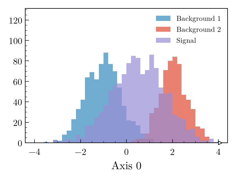
# Create histograms and fill them
h1 = hist.new.Reg(40, -4, 4).Weight().fill(np.random.normal(-1, 0.8, 800))
h2 = hist.new.Reg(40, -4, 4).Weight().fill(np.random.normal(2, 0.6, 600))
h3 = hist.new.Reg(40, -4, 4).Weight().fill(np.random.normal(0.5, 1.2, 1200))

fig, ax = plt.subplots()
mh.histplot(
 [h1, h2, h3],
 histtype='fill',
 stack=True,
 label=['Background 1', 'Background 2', 'Signal'],
 ax=ax
)
ax.legend(loc='upper right')
mh.yscale_legend(soft_fail=True)
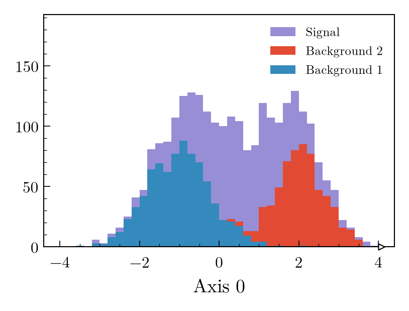
# Create histograms and fill them
h1 = hist.new.Reg(40, -4, 4).Weight().fill(np.random.normal(-1, 0.8, 800))
h2 = hist.new.Reg(40, -4, 4).Weight().fill(np.random.normal(2, 0.6, 600))
h3 = hist.new.Reg(40, -4, 4).Weight().fill(np.random.normal(0.5, 1.2, 1200))

fig, ax = plt.subplots()
mh.histplot(
 [h1, h2, h3],
 histtype='fill',
 stack=True,
 sort='yield',
 label=['Background 1', 'Background 2', 'Signal'],
 ax=ax
)
ax.legend(loc='upper right')
mh.yscale_legend(soft_fail=True)
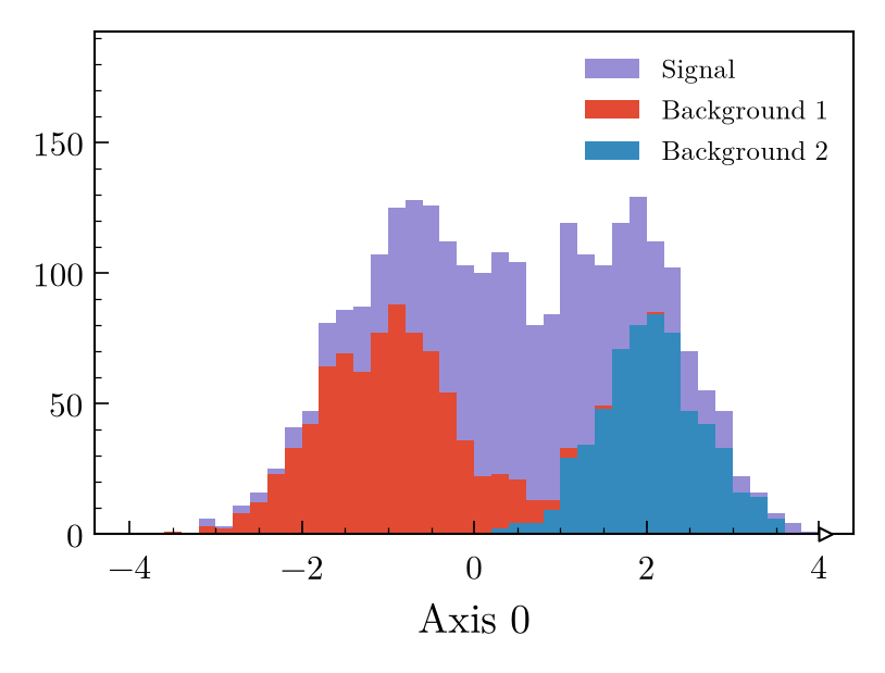
# Create histograms and fill them
h1 = hist.new.Reg(40, -4, 4).Weight().fill(np.random.normal(-1, 0.8, 800))
h2 = hist.new.Reg(40, -4, 4).Weight().fill(np.random.normal(2, 0.6, 600))
h3 = hist.new.Reg(40, -4, 4).Weight().fill(np.random.normal(0.5, 1.2, 1200))

fig, ax = plt.subplots()
mh.histplot(
 [h1, h2, h3],
 histtype='fill',
 stack=True,
 sort='label',
 label=['Background 1', 'Background 2', 'Signal'],
 ax=ax
)
ax.legend(loc='upper right')
mh.yscale_legend(soft_fail=True)
# Create histograms and fill them
h1 = hist.new.Reg(40, -4, 4).Weight().fill(np.random.normal(-1, 0.8, 800))
h2 = hist.new.Reg(40, -4, 4).Weight().fill(np.random.normal(2, 0.6, 600))
h3 = hist.new.Reg(40, -4, 4).Weight().fill(np.random.normal(0.5, 1.2, 1200))

fig, ax = plt.subplots()
mh.histplot(
 [h1, h2, h3],
 histtype='fill',
 stack=True,
 sort='l_r',
 label=['Background 1', 'Background 2', 'Signal'],
 ax=ax
)
ax.legend(loc='upper right')
mh.yscale_legend(soft_fail=True)
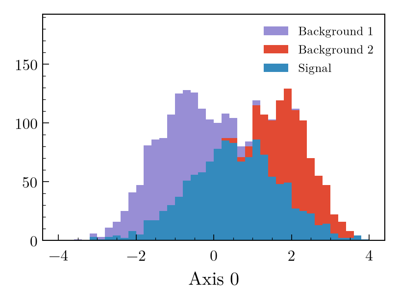
# Create histograms and fill them
h1 = hist.new.Reg(40, -4, 4).Weight().fill(np.random.normal(-1, 0.8, 800))
h2 = hist.new.Reg(40, -4, 4).Weight().fill(np.random.normal(2, 0.6, 600))
h3 = hist.new.Reg(40, -4, 4).Weight().fill(np.random.normal(0.5, 1.2, 1200))

fig, ax = plt.subplots()
mh.histplot(
 [h1, h2, h3],
 stack=True,
 label=['Background 1', 'Background 2', 'Signal'],
 ax=ax
)
txt_obj = mh.add_text('plothist', loc='over left')
ax.legend(loc='upper right')
mh.yscale_legend(soft_fail=True)
# Create histograms and fill them
h1 = hist.new.Reg(40, -4, 4).Weight().fill(np.random.normal(-1, 0.8, 800))
h2 = hist.new.Reg(40, -4, 4).Weight().fill(np.random.normal(2, 0.6, 600))
h3 = hist.new.Reg(40, -4, 4).Weight().fill(np.random.normal(0.5, 1.2, 1200))

fig, ax = plt.subplots()
mh.histplot(
 [h1, h2, h3],
 histtype='fill',
 alpha=0.7,
 label=['Background 1', 'Background 2', 'Signal'],
 ax=ax
)
ax.legend(loc='upper right')
mh.yscale_legend(soft_fail=True)
# Create histograms and fill them
h1 = hist.new.Reg(40, -4, 4).Weight().fill(np.random.normal(-1, 0.8, 800))
h2 = hist.new.Reg(40, -4, 4).Weight().fill(np.random.normal(2, 0.6, 600))
h3 = hist.new.Reg(40, -4, 4).Weight().fill(np.random.normal(0.5, 1.2, 1200))

fig, ax = plt.subplots()
mh.histplot(
 [h1, h2, h3],
 histtype='fill',
 stack=True,
 label=['Background 1', 'Background 2', 'Signal'],
 ax=ax
)
ax.legend(loc='upper right')
mh.yscale_legend(soft_fail=True)
# Create histograms and fill them
h1 = hist.new.Reg(40, -4, 4).Weight().fill(np.random.normal(-1, 0.8, 800))
h2 = hist.new.Reg(40, -4, 4).Weight().fill(np.random.normal(2, 0.6, 600))
h3 = hist.new.Reg(40, -4, 4).Weight().fill(np.random.normal(0.5, 1.2, 1200))

fig, ax = plt.subplots()
mh.histplot(
 [h1, h2, h3],
 histtype='fill',
 stack=True,
 sort='yield',
 label=['Background 1', 'Background 2', 'Signal'],
 ax=ax
)
ax.legend(loc='upper right')
mh.yscale_legend(soft_fail=True)
# Create histograms and fill them
h1 = hist.new.Reg(40, -4, 4).Weight().fill(np.random.normal(-1, 0.8, 800))
h2 = hist.new.Reg(40, -4, 4).Weight().fill(np.random.normal(2, 0.6, 600))
h3 = hist.new.Reg(40, -4, 4).Weight().fill(np.random.normal(0.5, 1.2, 1200))

fig, ax = plt.subplots()
mh.histplot(
 [h1, h2, h3],
 histtype='fill',
 stack=True,
 sort='label',
 label=['Background 1', 'Background 2', 'Signal'],
 ax=ax
)
ax.legend(loc='upper right')
mh.yscale_legend(soft_fail=True)
# Create histograms and fill them
h1 = hist.new.Reg(40, -4, 4).Weight().fill(np.random.normal(-1, 0.8, 800))
h2 = hist.new.Reg(40, -4, 4).Weight().fill(np.random.normal(2, 0.6, 600))
h3 = hist.new.Reg(40, -4, 4).Weight().fill(np.random.normal(0.5, 1.2, 1200))

fig, ax = plt.subplots()
mh.histplot(
 [h1, h2, h3],
 histtype='fill',
 stack=True,
 sort='l_r',
 label=['Background 1', 'Background 2', 'Signal'],
 ax=ax
)
ax.legend(loc='upper right')
mh.yscale_legend(soft_fail=True)
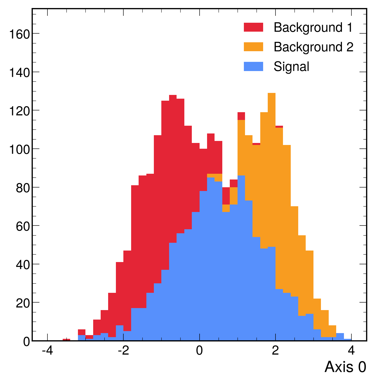
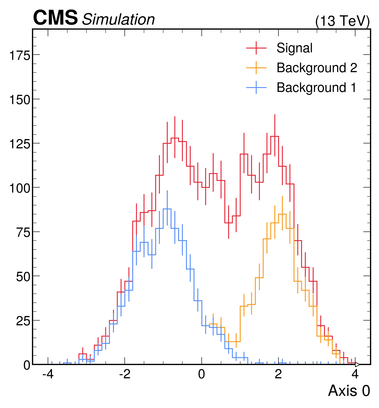
# Create histograms and fill them
h1 = hist.new.Reg(40, -4, 4).Weight().fill(np.random.normal(-1, 0.8, 800))
h2 = hist.new.Reg(40, -4, 4).Weight().fill(np.random.normal(2, 0.6, 600))
h3 = hist.new.Reg(40, -4, 4).Weight().fill(np.random.normal(0.5, 1.2, 1200))

fig, ax = plt.subplots()
mh.histplot(
 [h1, h2, h3],
 stack=True,
 label=['Background 1', 'Background 2', 'Signal'],
 ax=ax
)
mh.cms.label(data=False)
ax.legend(loc='upper right')
mh.yscale_legend(soft_fail=True)
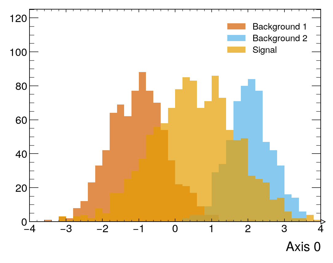
# Create histograms and fill them
h1 = hist.new.Reg(40, -4, 4).Weight().fill(np.random.normal(-1, 0.8, 800))
h2 = hist.new.Reg(40, -4, 4).Weight().fill(np.random.normal(2, 0.6, 600))
h3 = hist.new.Reg(40, -4, 4).Weight().fill(np.random.normal(0.5, 1.2, 1200))

fig, ax = plt.subplots()
mh.histplot(
 [h1, h2, h3],
 histtype='fill',
 alpha=0.7,
 label=['Background 1', 'Background 2', 'Signal'],
 ax=ax
)
ax.legend(loc='upper right')
mh.yscale_legend(soft_fail=True)
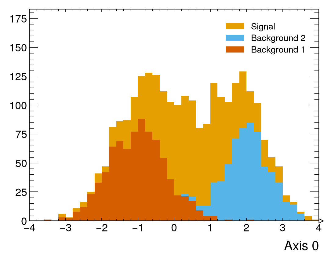
# Create histograms and fill them
h1 = hist.new.Reg(40, -4, 4).Weight().fill(np.random.normal(-1, 0.8, 800))
h2 = hist.new.Reg(40, -4, 4).Weight().fill(np.random.normal(2, 0.6, 600))
h3 = hist.new.Reg(40, -4, 4).Weight().fill(np.random.normal(0.5, 1.2, 1200))

fig, ax = plt.subplots()
mh.histplot(
 [h1, h2, h3],
 histtype='fill',
 stack=True,
 label=['Background 1', 'Background 2', 'Signal'],
 ax=ax
)
ax.legend(loc='upper right')
mh.yscale_legend(soft_fail=True)
# Create histograms and fill them
h1 = hist.new.Reg(40, -4, 4).Weight().fill(np.random.normal(-1, 0.8, 800))
h2 = hist.new.Reg(40, -4, 4).Weight().fill(np.random.normal(2, 0.6, 600))
h3 = hist.new.Reg(40, -4, 4).Weight().fill(np.random.normal(0.5, 1.2, 1200))

fig, ax = plt.subplots()
mh.histplot(
 [h1, h2, h3],
 histtype='fill',
 stack=True,
 sort='yield',
 label=['Background 1', 'Background 2', 'Signal'],
 ax=ax
)
ax.legend(loc='upper right')
mh.yscale_legend(soft_fail=True)
# Create histograms and fill them
h1 = hist.new.Reg(40, -4, 4).Weight().fill(np.random.normal(-1, 0.8, 800))
h2 = hist.new.Reg(40, -4, 4).Weight().fill(np.random.normal(2, 0.6, 600))
h3 = hist.new.Reg(40, -4, 4).Weight().fill(np.random.normal(0.5, 1.2, 1200))

fig, ax = plt.subplots()
mh.histplot(
 [h1, h2, h3],
 histtype='fill',
 stack=True,
 sort='label',
 label=['Background 1', 'Background 2', 'Signal'],
 ax=ax
)
ax.legend(loc='upper right')
mh.yscale_legend(soft_fail=True)
# Create histograms and fill them
h1 = hist.new.Reg(40, -4, 4).Weight().fill(np.random.normal(-1, 0.8, 800))
h2 = hist.new.Reg(40, -4, 4).Weight().fill(np.random.normal(2, 0.6, 600))
h3 = hist.new.Reg(40, -4, 4).Weight().fill(np.random.normal(0.5, 1.2, 1200))

fig, ax = plt.subplots()
mh.histplot(
 [h1, h2, h3],
 histtype='fill',
 stack=True,
 sort='l_r',
 label=['Background 1', 'Background 2', 'Signal'],
 ax=ax
)
ax.legend(loc='upper right')
mh.yscale_legend(soft_fail=True)
# Create histograms and fill them
h1 = hist.new.Reg(40, -4, 4).Weight().fill(np.random.normal(-1, 0.8, 800))
h2 = hist.new.Reg(40, -4, 4).Weight().fill(np.random.normal(2, 0.6, 600))
h3 = hist.new.Reg(40, -4, 4).Weight().fill(np.random.normal(0.5, 1.2, 1200))

fig, ax = plt.subplots()
mh.histplot(
 [h1, h2, h3],
 stack=True,
 label=['Background 1', 'Background 2', 'Signal'],
 ax=ax
)
mh.atlas.label(data=False)
mh.mpl_magic(soft_fail=True)
ax.legend(loc='upper right')
mh.yscale_legend(soft_fail=True)
# Create histograms and fill them
h1 = hist.new.Reg(40, -4, 4).Weight().fill(np.random.normal(-1, 0.8, 800))
h2 = hist.new.Reg(40, -4, 4).Weight().fill(np.random.normal(2, 0.6, 600))
h3 = hist.new.Reg(40, -4, 4).Weight().fill(np.random.normal(0.5, 1.2, 1200))

fig, ax = plt.subplots()
mh.histplot(
 [h1, h2, h3],
 histtype='fill',
 alpha=0.7,
 label=['Background 1', 'Background 2', 'Signal'],
 ax=ax
)
ax.legend(loc='upper right')
mh.yscale_legend(soft_fail=True)
# Create histograms and fill them
h1 = hist.new.Reg(40, -4, 4).Weight().fill(np.random.normal(-1, 0.8, 800))
h2 = hist.new.Reg(40, -4, 4).Weight().fill(np.random.normal(2, 0.6, 600))
h3 = hist.new.Reg(40, -4, 4).Weight().fill(np.random.normal(0.5, 1.2, 1200))

fig, ax = plt.subplots()
mh.histplot(
 [h1, h2, h3],
 histtype='fill',
 stack=True,
 label=['Background 1', 'Background 2', 'Signal'],
 ax=ax
)
ax.legend(loc='upper right')
mh.yscale_legend(soft_fail=True)
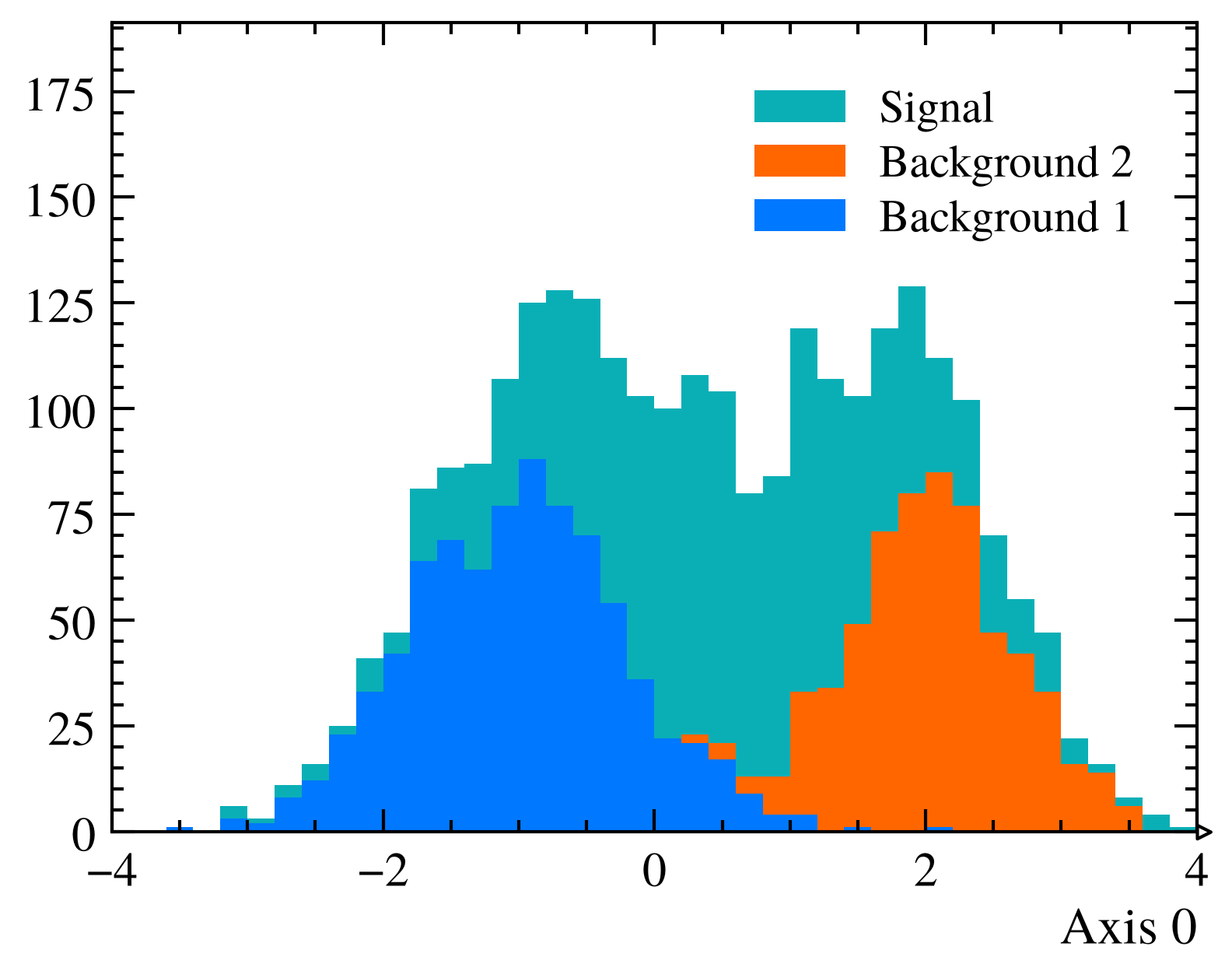
# Create histograms and fill them
h1 = hist.new.Reg(40, -4, 4).Weight().fill(np.random.normal(-1, 0.8, 800))
h2 = hist.new.Reg(40, -4, 4).Weight().fill(np.random.normal(2, 0.6, 600))
h3 = hist.new.Reg(40, -4, 4).Weight().fill(np.random.normal(0.5, 1.2, 1200))

fig, ax = plt.subplots()
mh.histplot(
 [h1, h2, h3],
 histtype='fill',
 stack=True,
 sort='yield',
 label=['Background 1', 'Background 2', 'Signal'],
 ax=ax
)
ax.legend(loc='upper right')
mh.yscale_legend(soft_fail=True)
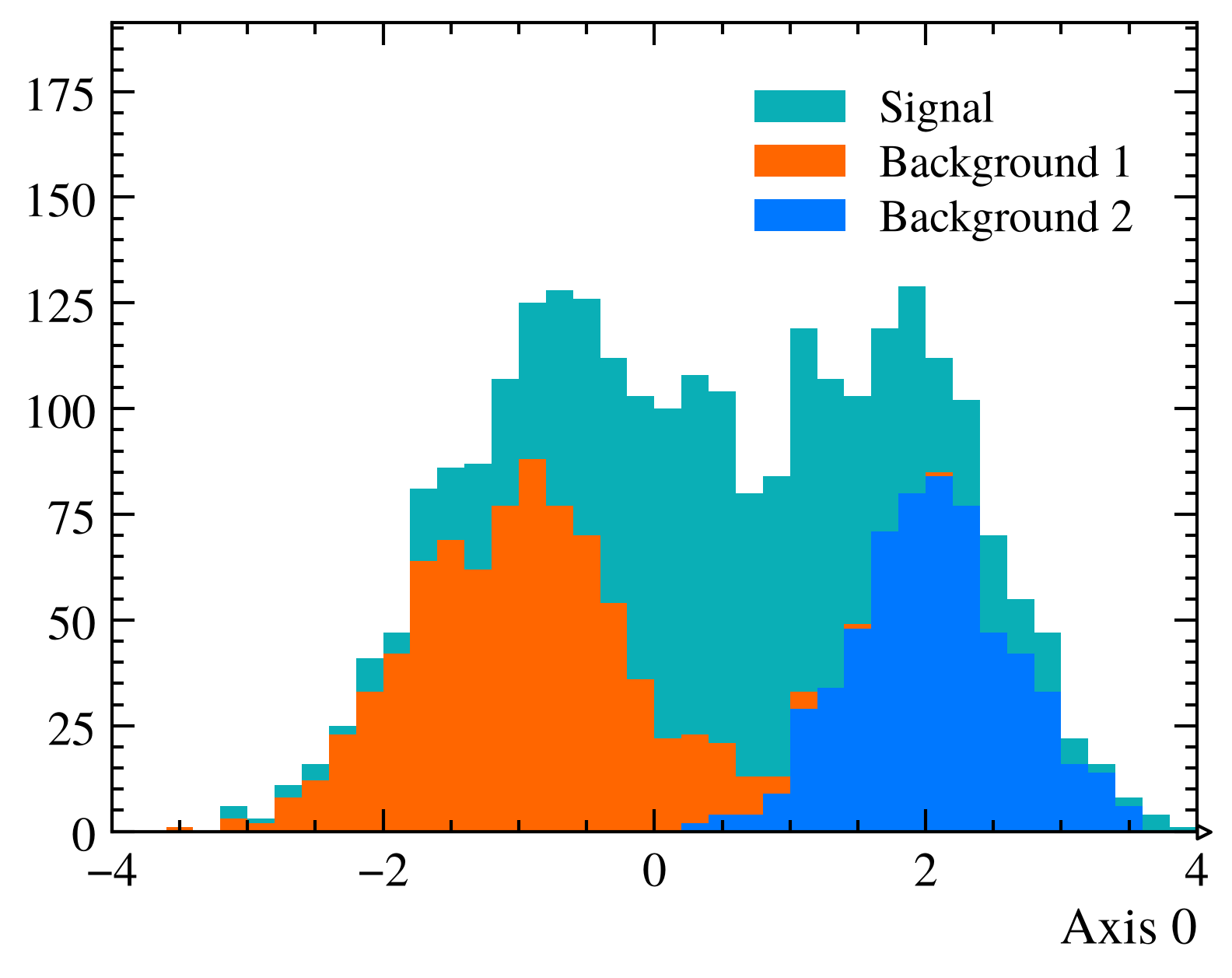
# Create histograms and fill them
h1 = hist.new.Reg(40, -4, 4).Weight().fill(np.random.normal(-1, 0.8, 800))
h2 = hist.new.Reg(40, -4, 4).Weight().fill(np.random.normal(2, 0.6, 600))
h3 = hist.new.Reg(40, -4, 4).Weight().fill(np.random.normal(0.5, 1.2, 1200))

fig, ax = plt.subplots()
mh.histplot(
 [h1, h2, h3],
 histtype='fill',
 stack=True,
 sort='label',
 label=['Background 1', 'Background 2', 'Signal'],
 ax=ax
)
ax.legend(loc='upper right')
mh.yscale_legend(soft_fail=True)
# Create histograms and fill them
h1 = hist.new.Reg(40, -4, 4).Weight().fill(np.random.normal(-1, 0.8, 800))
h2 = hist.new.Reg(40, -4, 4).Weight().fill(np.random.normal(2, 0.6, 600))
h3 = hist.new.Reg(40, -4, 4).Weight().fill(np.random.normal(0.5, 1.2, 1200))

fig, ax = plt.subplots()
mh.histplot(
 [h1, h2, h3],
 histtype='fill',
 stack=True,
 sort='l_r',
 label=['Background 1', 'Background 2', 'Signal'],
 ax=ax
)
ax.legend(loc='upper right')
mh.yscale_legend(soft_fail=True)
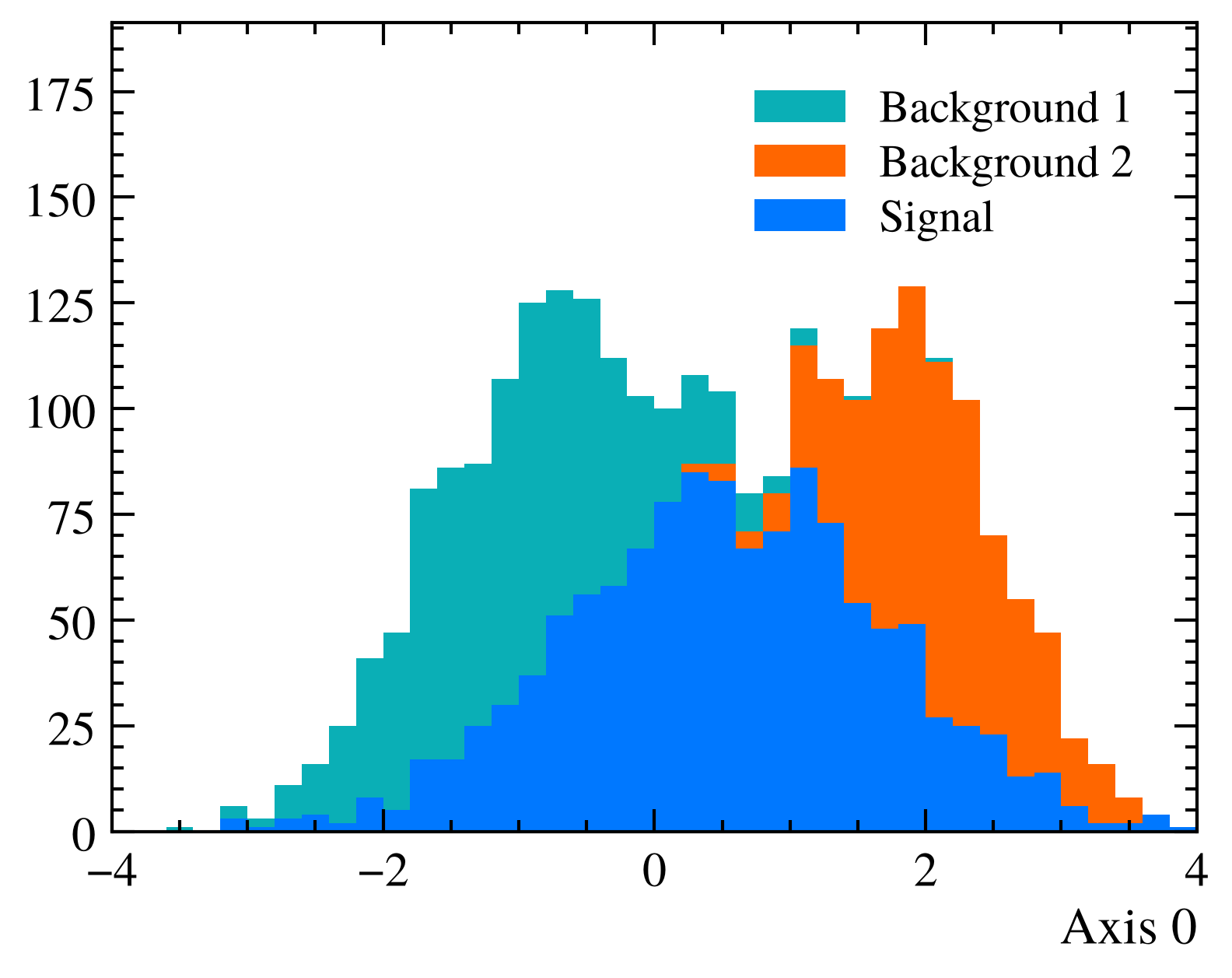
# Create histograms and fill them
h1 = hist.new.Reg(40, -4, 4).Weight().fill(np.random.normal(-1, 0.8, 800))
h2 = hist.new.Reg(40, -4, 4).Weight().fill(np.random.normal(2, 0.6, 600))
h3 = hist.new.Reg(40, -4, 4).Weight().fill(np.random.normal(0.5, 1.2, 1200))

fig, ax = plt.subplots()
mh.histplot(
 [h1, h2, h3],
 stack=True,
 label=['Background 1', 'Background 2', 'Signal'],
 ax=ax
)
mh.lhcb.label(data=False)
ax.legend(loc='upper right')
mh.yscale_legend(soft_fail=True)
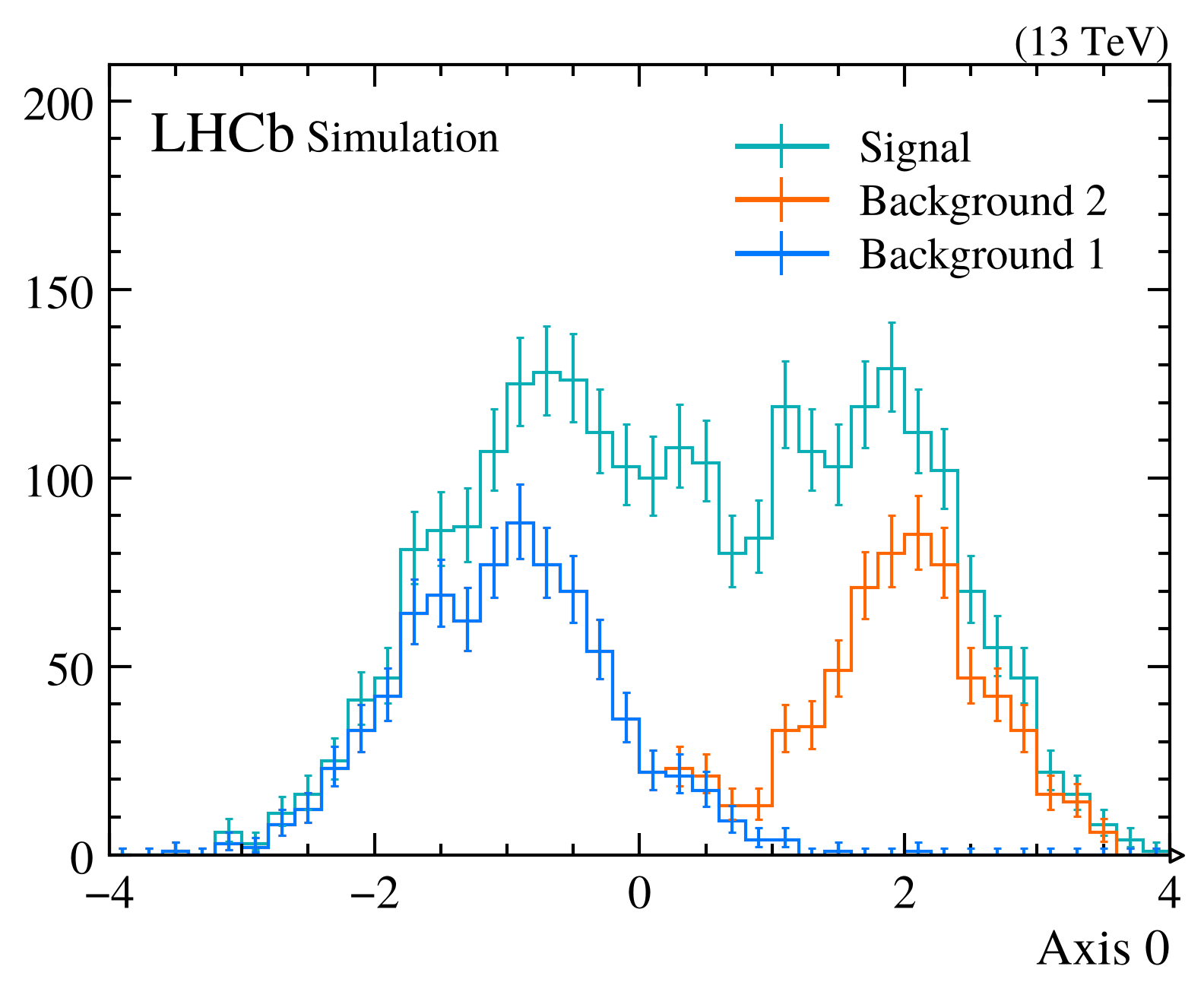
# Create histograms and fill them
h1 = hist.new.Reg(40, -4, 4).Weight().fill(np.random.normal(-1, 0.8, 800))
h2 = hist.new.Reg(40, -4, 4).Weight().fill(np.random.normal(2, 0.6, 600))
h3 = hist.new.Reg(40, -4, 4).Weight().fill(np.random.normal(0.5, 1.2, 1200))

fig, ax = plt.subplots()
mh.histplot(
 [h1, h2, h3],
 histtype='fill',
 alpha=0.7,
 label=['Background 1', 'Background 2', 'Signal'],
 ax=ax
)
ax.legend(loc='upper right')
mh.yscale_legend(soft_fail=True)
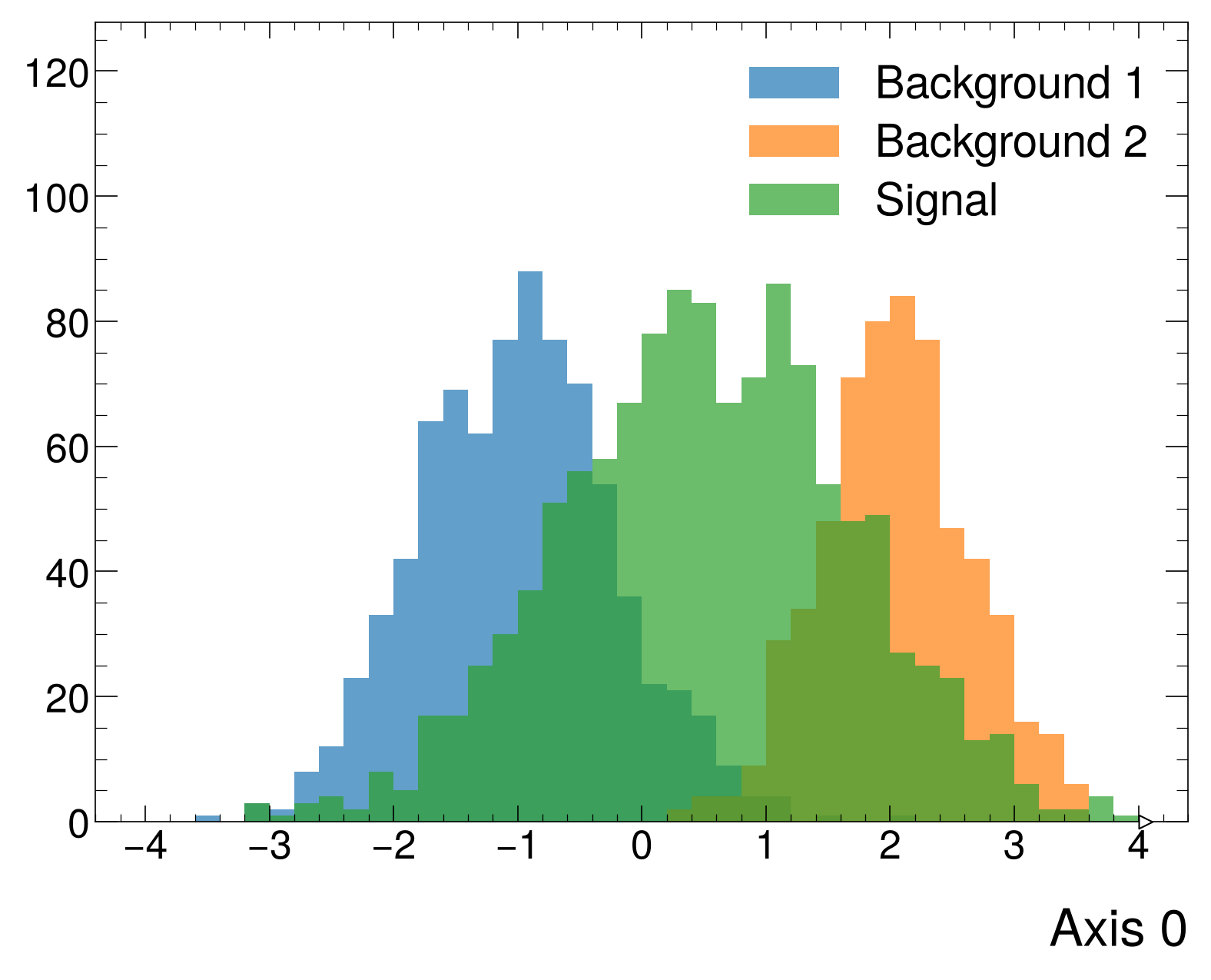
# Create histograms and fill them
h1 = hist.new.Reg(40, -4, 4).Weight().fill(np.random.normal(-1, 0.8, 800))
h2 = hist.new.Reg(40, -4, 4).Weight().fill(np.random.normal(2, 0.6, 600))
h3 = hist.new.Reg(40, -4, 4).Weight().fill(np.random.normal(0.5, 1.2, 1200))

fig, ax = plt.subplots()
mh.histplot(
 [h1, h2, h3],
 histtype='fill',
 stack=True,
 label=['Background 1', 'Background 2', 'Signal'],
 ax=ax
)
ax.legend(loc='upper right')
mh.yscale_legend(soft_fail=True)
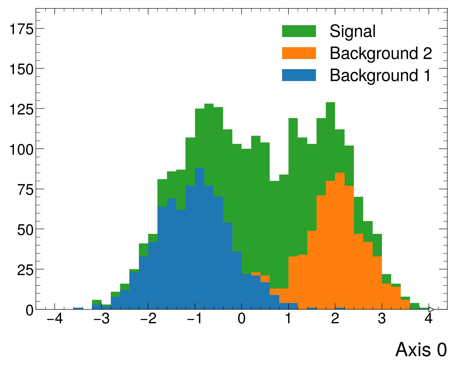
# Create histograms and fill them
h1 = hist.new.Reg(40, -4, 4).Weight().fill(np.random.normal(-1, 0.8, 800))
h2 = hist.new.Reg(40, -4, 4).Weight().fill(np.random.normal(2, 0.6, 600))
h3 = hist.new.Reg(40, -4, 4).Weight().fill(np.random.normal(0.5, 1.2, 1200))

fig, ax = plt.subplots()
mh.histplot(
 [h1, h2, h3],
 histtype='fill',
 stack=True,
 sort='yield',
 label=['Background 1', 'Background 2', 'Signal'],
 ax=ax
)
ax.legend(loc='upper right')
mh.yscale_legend(soft_fail=True)
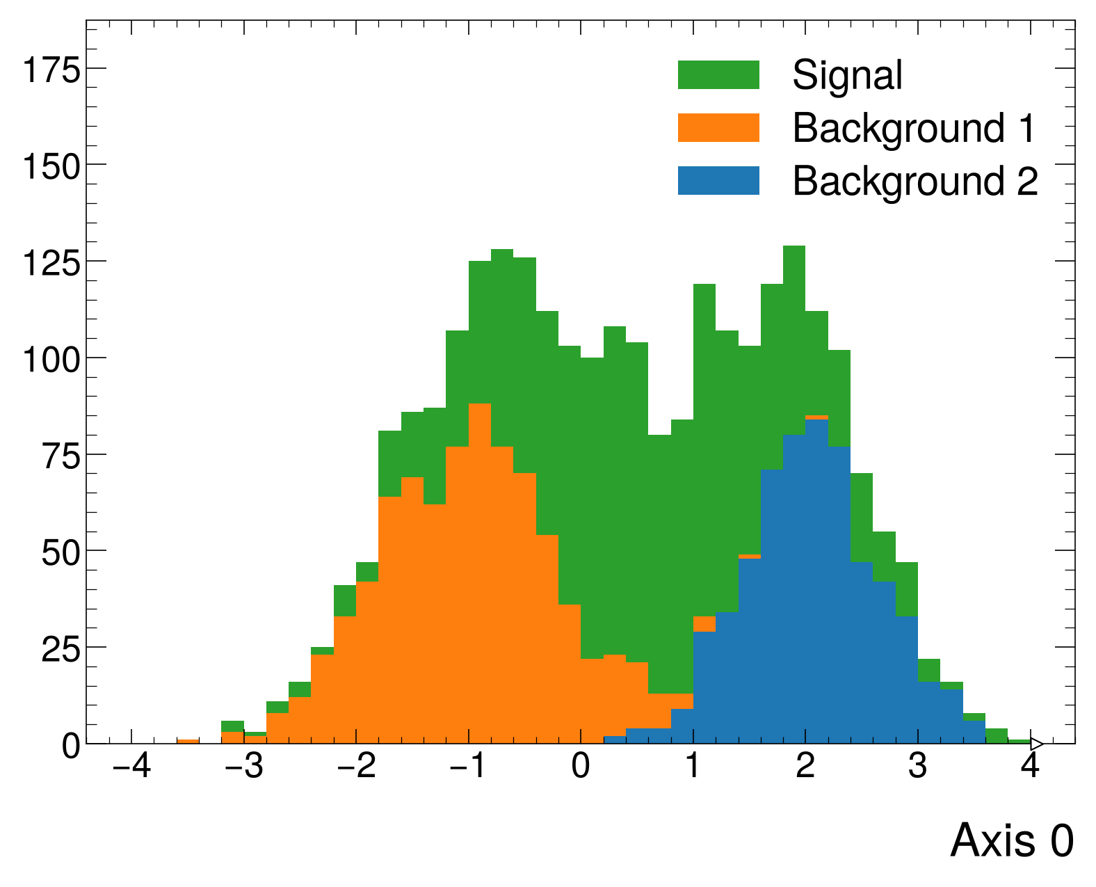
# Create histograms and fill them
h1 = hist.new.Reg(40, -4, 4).Weight().fill(np.random.normal(-1, 0.8, 800))
h2 = hist.new.Reg(40, -4, 4).Weight().fill(np.random.normal(2, 0.6, 600))
h3 = hist.new.Reg(40, -4, 4).Weight().fill(np.random.normal(0.5, 1.2, 1200))

fig, ax = plt.subplots()
mh.histplot(
 [h1, h2, h3],
 histtype='fill',
 stack=True,
 sort='label',
 label=['Background 1', 'Background 2', 'Signal'],
 ax=ax
)
ax.legend(loc='upper right')
mh.yscale_legend(soft_fail=True)
# Create histograms and fill them
h1 = hist.new.Reg(40, -4, 4).Weight().fill(np.random.normal(-1, 0.8, 800))
h2 = hist.new.Reg(40, -4, 4).Weight().fill(np.random.normal(2, 0.6, 600))
h3 = hist.new.Reg(40, -4, 4).Weight().fill(np.random.normal(0.5, 1.2, 1200))

fig, ax = plt.subplots()
mh.histplot(
 [h1, h2, h3],
 histtype='fill',
 stack=True,
 sort='l_r',
 label=['Background 1', 'Background 2', 'Signal'],
 ax=ax
)
ax.legend(loc='upper right')
mh.yscale_legend(soft_fail=True)
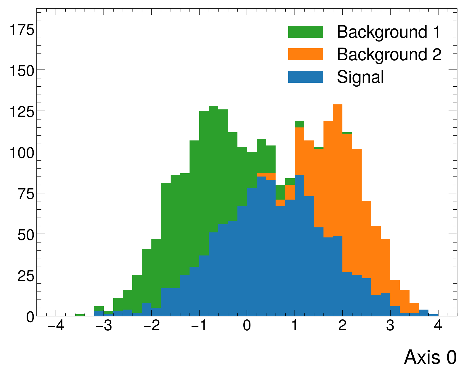
# Create histograms and fill them
h1 = hist.new.Reg(40, -4, 4).Weight().fill(np.random.normal(-1, 0.8, 800))
h2 = hist.new.Reg(40, -4, 4).Weight().fill(np.random.normal(2, 0.6, 600))
h3 = hist.new.Reg(40, -4, 4).Weight().fill(np.random.normal(0.5, 1.2, 1200))

fig, ax = plt.subplots()
mh.histplot(
 [h1, h2, h3],
 stack=True,
 label=['Background 1', 'Background 2', 'Signal'],
 ax=ax
)
mh.alice.label(data=False)
mh.mpl_magic(soft_fail=True)
ax.legend(loc='upper right')
mh.yscale_legend(soft_fail=True)
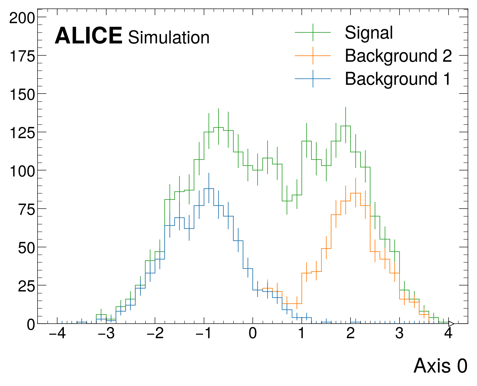
# Create histograms and fill them
h1 = hist.new.Reg(40, -4, 4).Weight().fill(np.random.normal(-1, 0.8, 800))
h2 = hist.new.Reg(40, -4, 4).Weight().fill(np.random.normal(2, 0.6, 600))
h3 = hist.new.Reg(40, -4, 4).Weight().fill(np.random.normal(0.5, 1.2, 1200))

fig, ax = plt.subplots()
mh.histplot(
 [h1, h2, h3],
 histtype='fill',
 alpha=0.7,
 label=['Background 1', 'Background 2', 'Signal'],
 ax=ax
)
ax.legend(loc='upper right')
mh.yscale_legend(soft_fail=True)
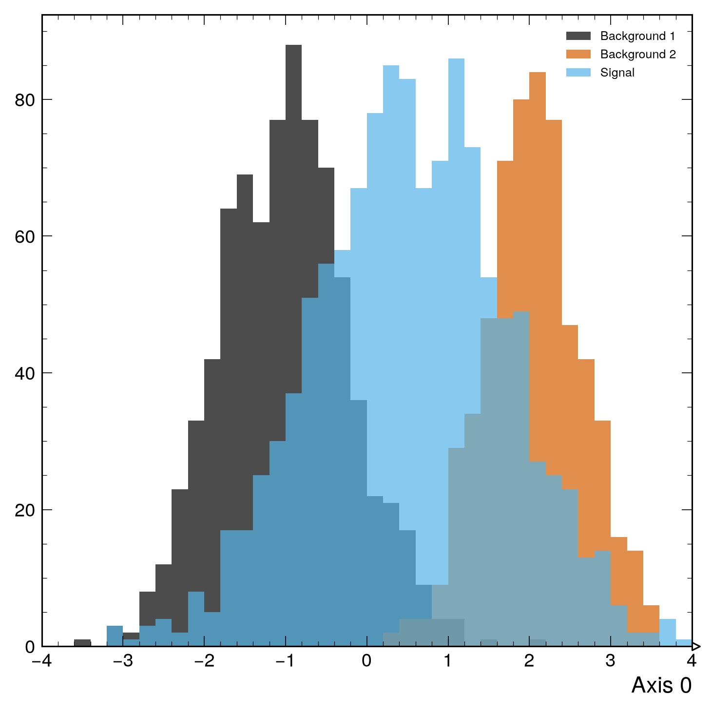
# Create histograms and fill them
h1 = hist.new.Reg(40, -4, 4).Weight().fill(np.random.normal(-1, 0.8, 800))
h2 = hist.new.Reg(40, -4, 4).Weight().fill(np.random.normal(2, 0.6, 600))
h3 = hist.new.Reg(40, -4, 4).Weight().fill(np.random.normal(0.5, 1.2, 1200))

fig, ax = plt.subplots()
mh.histplot(
 [h1, h2, h3],
 histtype='fill',
 stack=True,
 label=['Background 1', 'Background 2', 'Signal'],
 ax=ax
)
ax.legend(loc='upper right')
mh.yscale_legend(soft_fail=True)
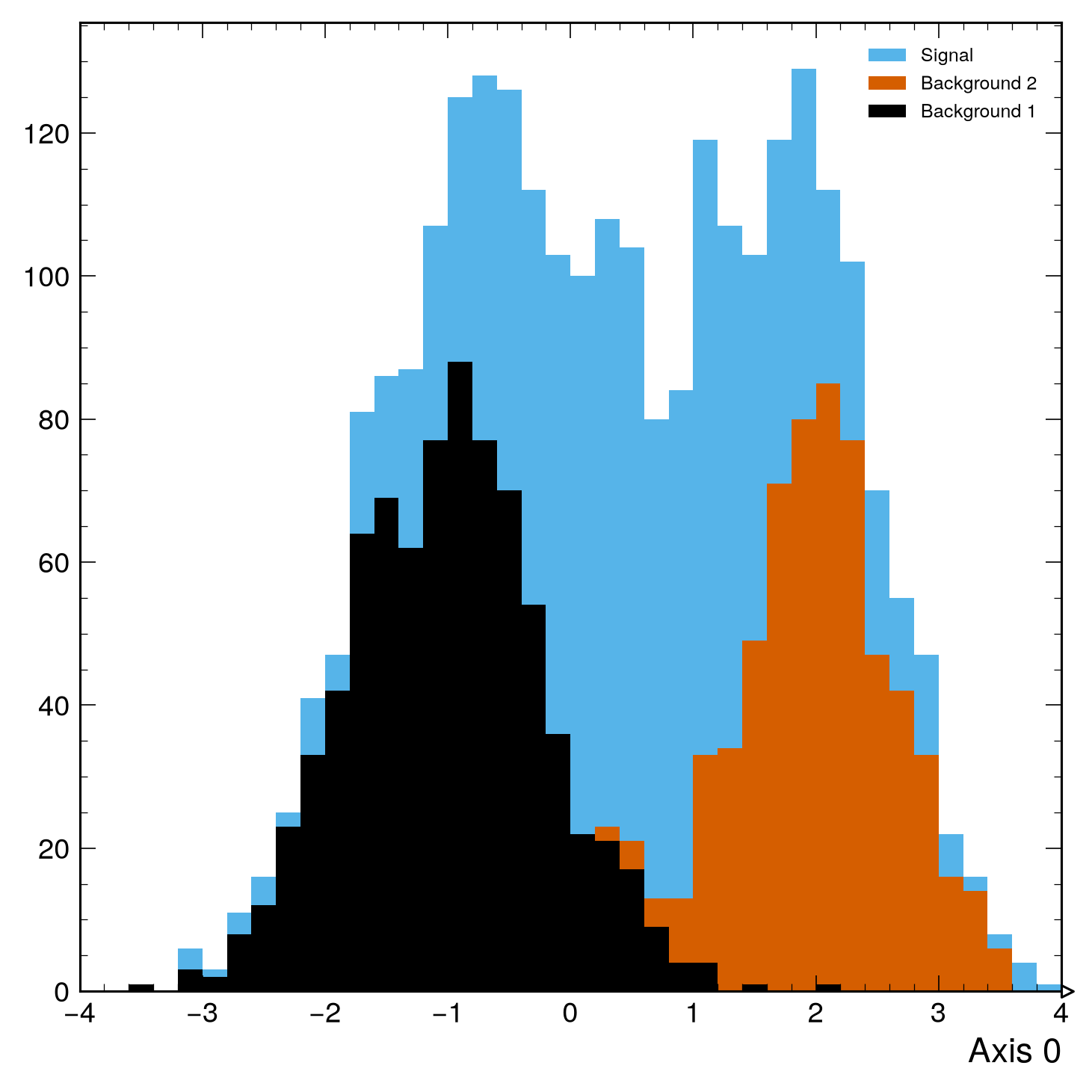
# Create histograms and fill them
h1 = hist.new.Reg(40, -4, 4).Weight().fill(np.random.normal(-1, 0.8, 800))
h2 = hist.new.Reg(40, -4, 4).Weight().fill(np.random.normal(2, 0.6, 600))
h3 = hist.new.Reg(40, -4, 4).Weight().fill(np.random.normal(0.5, 1.2, 1200))

fig, ax = plt.subplots()
mh.histplot(
 [h1, h2, h3],
 histtype='fill',
 stack=True,
 sort='yield',
 label=['Background 1', 'Background 2', 'Signal'],
 ax=ax
)
ax.legend(loc='upper right')
mh.yscale_legend(soft_fail=True)
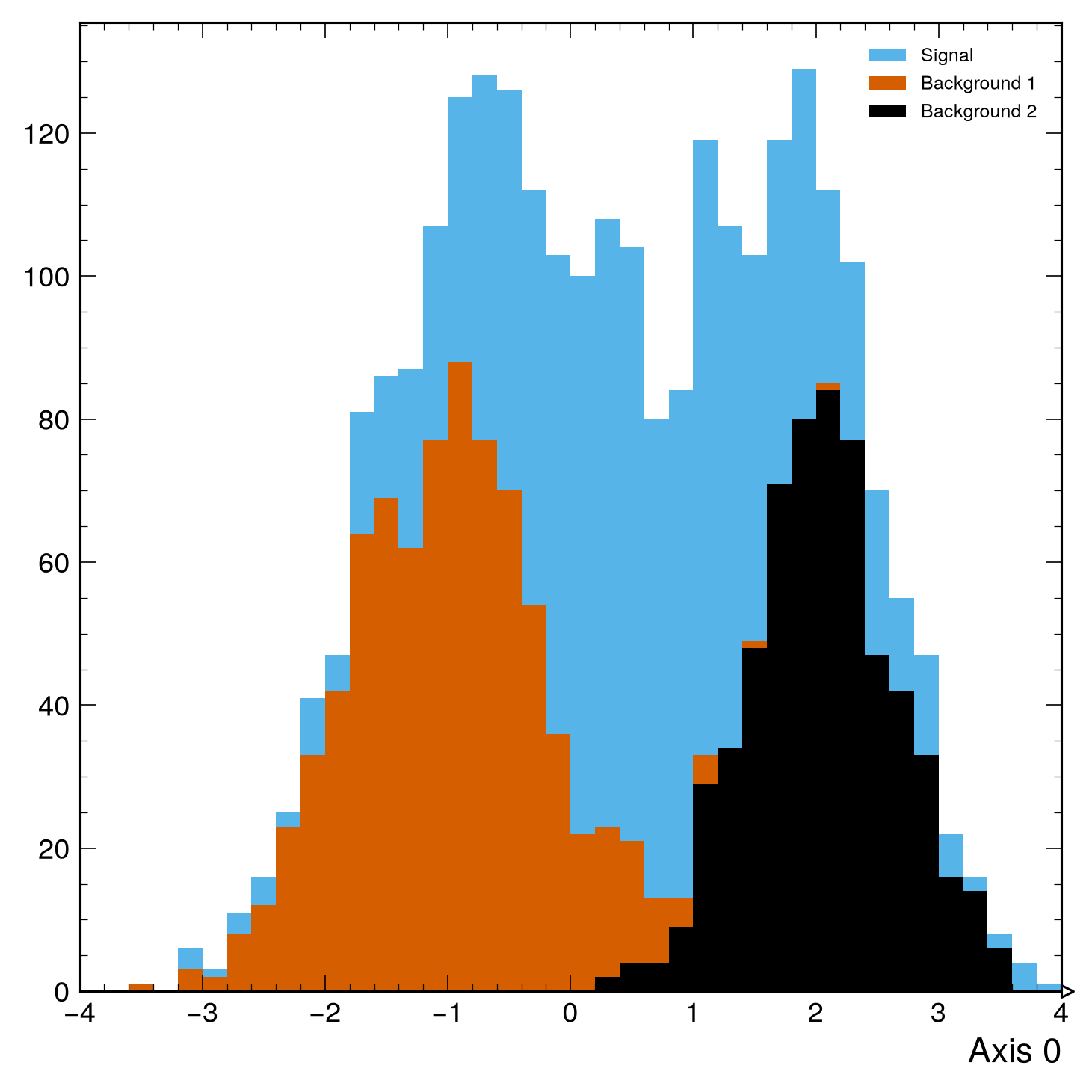
# Create histograms and fill them
h1 = hist.new.Reg(40, -4, 4).Weight().fill(np.random.normal(-1, 0.8, 800))
h2 = hist.new.Reg(40, -4, 4).Weight().fill(np.random.normal(2, 0.6, 600))
h3 = hist.new.Reg(40, -4, 4).Weight().fill(np.random.normal(0.5, 1.2, 1200))

fig, ax = plt.subplots()
mh.histplot(
 [h1, h2, h3],
 histtype='fill',
 stack=True,
 sort='label',
 label=['Background 1', 'Background 2', 'Signal'],
 ax=ax
)
ax.legend(loc='upper right')
mh.yscale_legend(soft_fail=True)
# Create histograms and fill them
h1 = hist.new.Reg(40, -4, 4).Weight().fill(np.random.normal(-1, 0.8, 800))
h2 = hist.new.Reg(40, -4, 4).Weight().fill(np.random.normal(2, 0.6, 600))
h3 = hist.new.Reg(40, -4, 4).Weight().fill(np.random.normal(0.5, 1.2, 1200))

fig, ax = plt.subplots()
mh.histplot(
 [h1, h2, h3],
 histtype='fill',
 stack=True,
 sort='l_r',
 label=['Background 1', 'Background 2', 'Signal'],
 ax=ax
)
ax.legend(loc='upper right')
mh.yscale_legend(soft_fail=True)
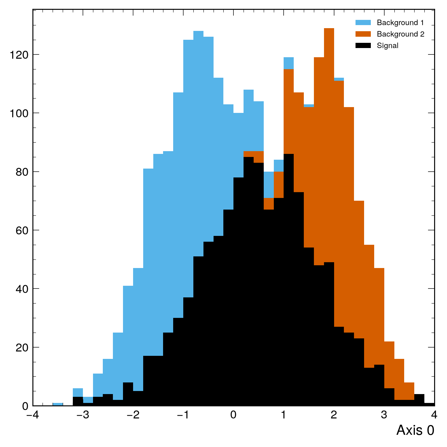
# Create histograms and fill them
h1 = hist.new.Reg(40, -4, 4).Weight().fill(np.random.normal(-1, 0.8, 800))
h2 = hist.new.Reg(40, -4, 4).Weight().fill(np.random.normal(2, 0.6, 600))
h3 = hist.new.Reg(40, -4, 4).Weight().fill(np.random.normal(0.5, 1.2, 1200))

fig, ax = plt.subplots()
mh.histplot(
 [h1, h2, h3],
 stack=True,
 label=['Background 1', 'Background 2', 'Signal'],
 ax=ax
)
mh.dune.label(data=False)
ax.legend(loc='upper right')
mh.yscale_legend(soft_fail=True)
Side by Side¤
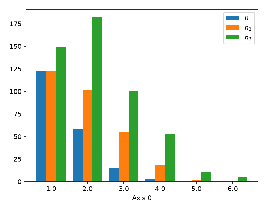
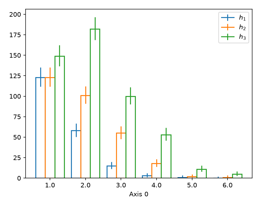
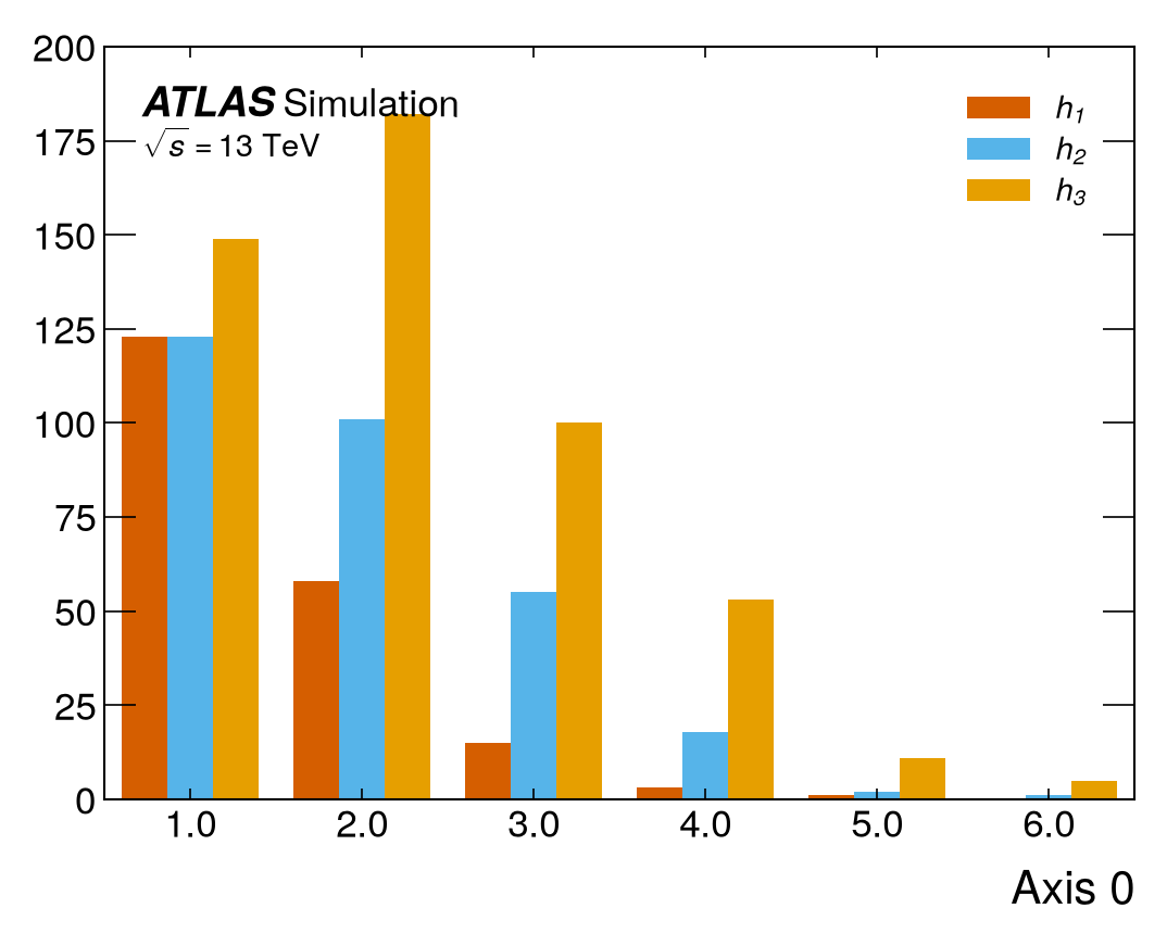
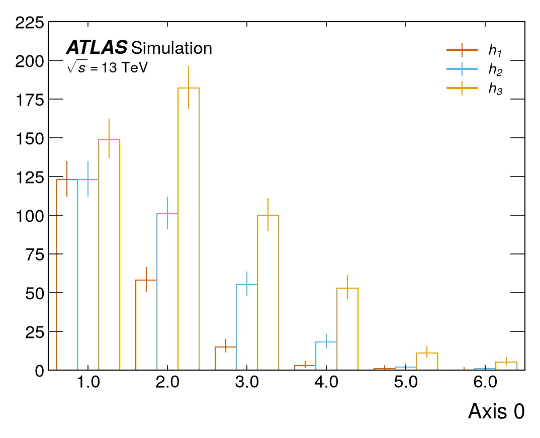
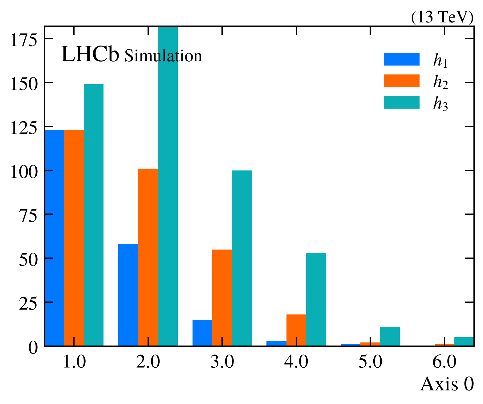
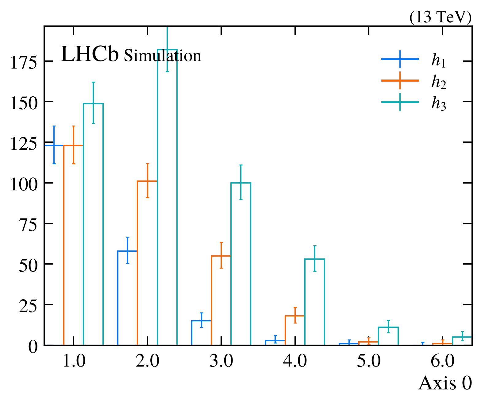
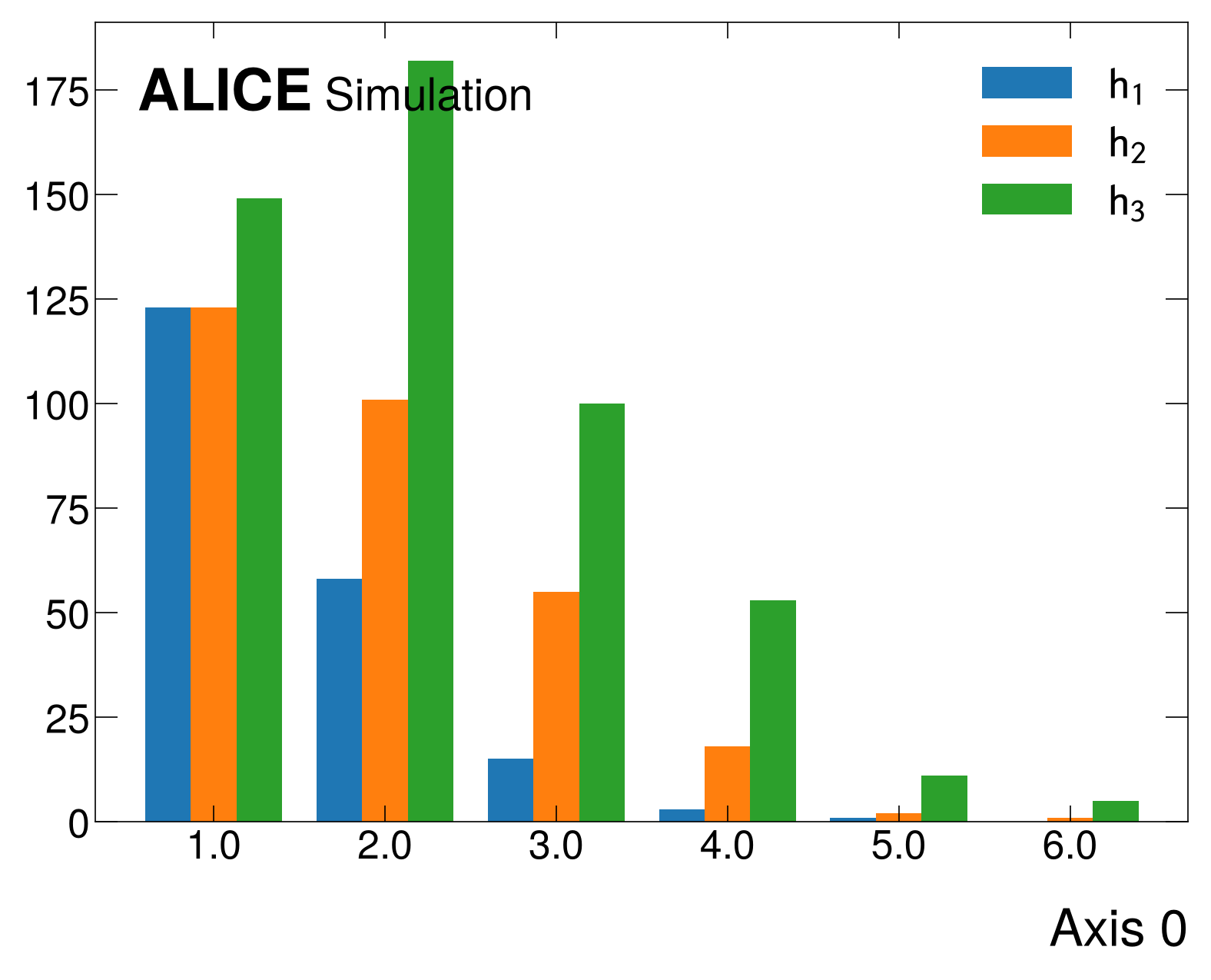
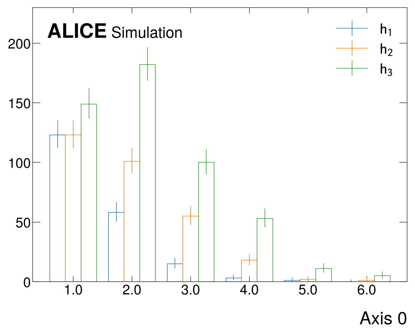
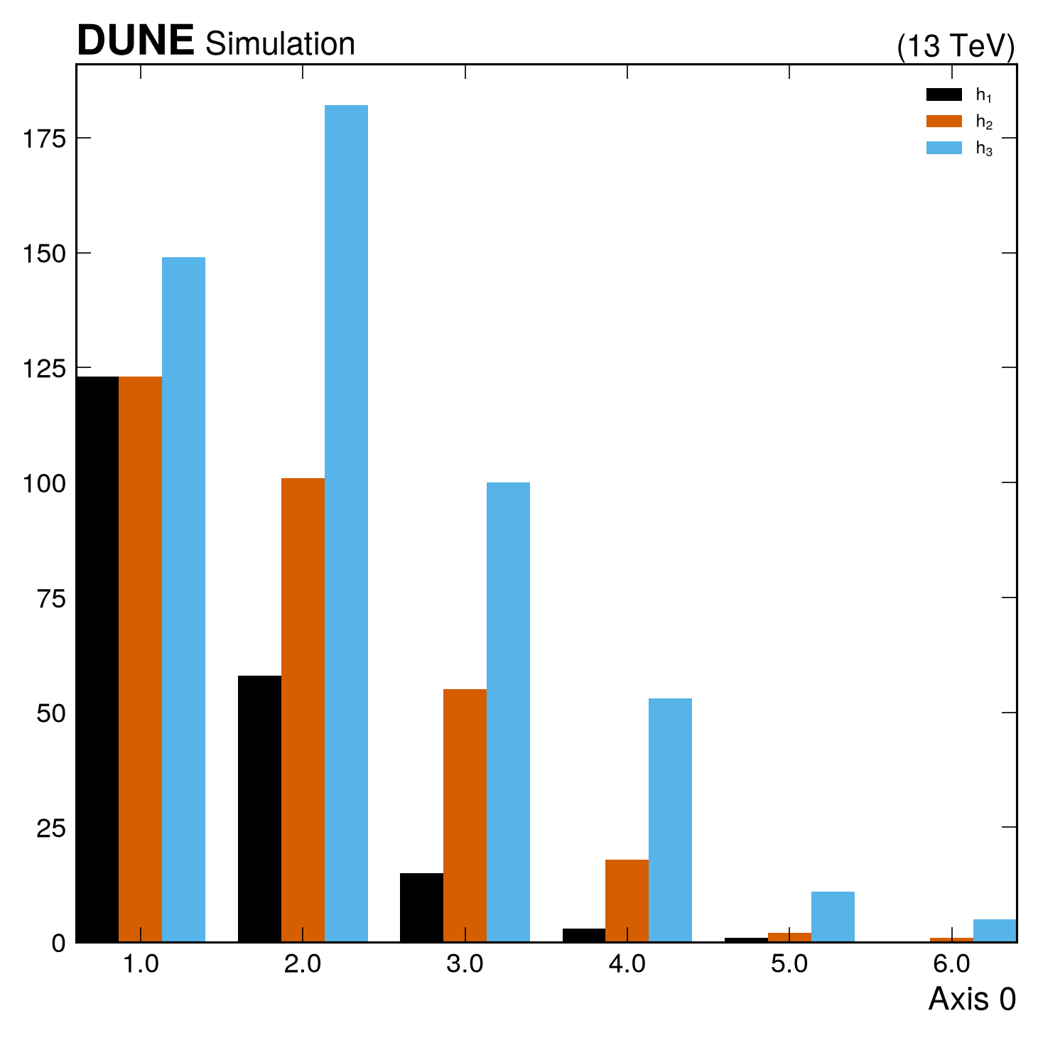
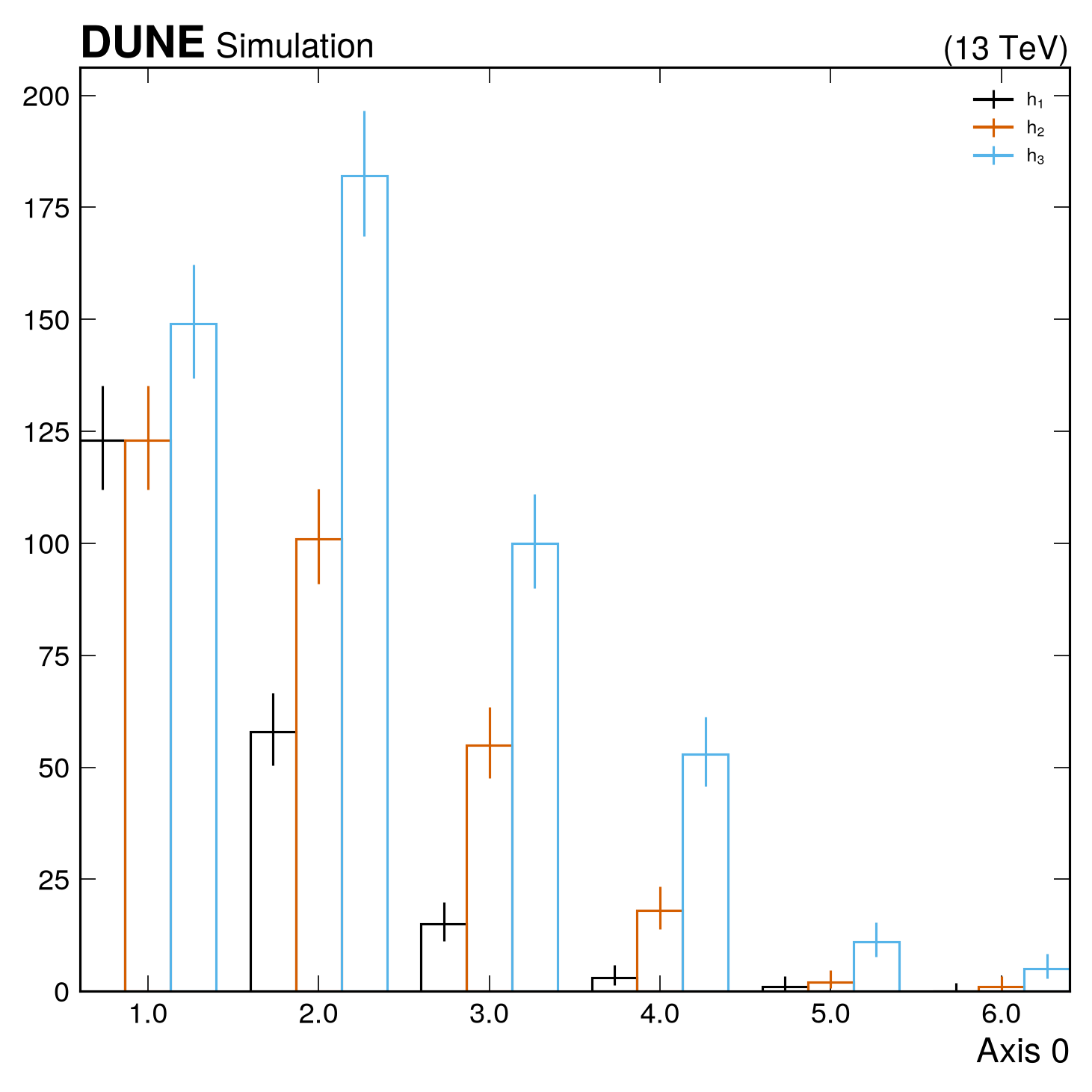
When plotting multiple histograms, the histtype can be set to 'bar' or 'barstep' to create side-by-side bar plots, just like matplotlib:
# Create histograms and fill them
h1 = hist.new.Reg(6, 0, 6).Weight().fill(np.random.poisson(0.5, 200))
h2 = hist.new.Reg(6, 0, 6).Weight().fill(np.random.poisson(1.0, 300))
h3 = hist.new.Reg(6, 0, 6).Weight().fill(np.random.poisson(1.2, 500))

fig, ax = plt.subplots()
mh.histplot(
 [h1, h2, h3],
 histtype='bar',
 label=['$h_1$', '$h_2$', '$h_3$'],
 ax=ax
)

ax.legend(loc='upper right')
mh.yscale_legend(soft_fail=True)
# Optional: move the x-ticks to the bin centers
ax.set_xticks(h1.axes[0].centers)
ax.set_xticklabels([x+0.5 for x in h1.axes[0].centers])
ax.minorticks_off()
# Create histograms and fill them
h1 = hist.new.Reg(6, 0, 6).Weight().fill(np.random.poisson(0.5, 200))
h2 = hist.new.Reg(6, 0, 6).Weight().fill(np.random.poisson(1.0, 300))
h3 = hist.new.Reg(6, 0, 6).Weight().fill(np.random.poisson(1.2, 500))

fig, ax = plt.subplots()
mh.histplot(
 [h1, h2, h3],
 histtype='barstep',
 label=['$h_1$', '$h_2$', '$h_3$'],
 ax=ax
)

ax.legend(loc='upper right')
mh.yscale_legend(soft_fail=True)
# Optional: move the x-ticks to the bin centers
ax.set_xticks(h1.axes[0].centers)
ax.set_xticklabels([x+0.5 for x in h1.axes[0].centers])
ax.minorticks_off()
# Create histograms and fill them
h1 = hist.new.Reg(6, 0, 6).Weight().fill(np.random.poisson(0.5, 200))
h2 = hist.new.Reg(6, 0, 6).Weight().fill(np.random.poisson(1.0, 300))
h3 = hist.new.Reg(6, 0, 6).Weight().fill(np.random.poisson(1.2, 500))

fig, ax = plt.subplots()
mh.histplot(
 [h1, h2, h3],
 histtype='bar',
 label=['$h_1$', '$h_2$', '$h_3$'],
 ax=ax
)
txt_obj = mh.add_text('plothist', loc='over left')
ax.legend(loc='upper right')
mh.yscale_legend(soft_fail=True)
# Optional: move the x-ticks to the bin centers
ax.set_xticks(h1.axes[0].centers)
ax.set_xticklabels([x+0.5 for x in h1.axes[0].centers])
ax.minorticks_off()
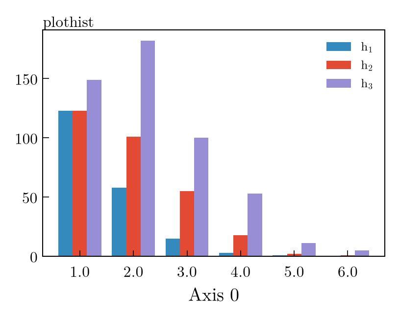
# Create histograms and fill them
h1 = hist.new.Reg(6, 0, 6).Weight().fill(np.random.poisson(0.5, 200))
h2 = hist.new.Reg(6, 0, 6).Weight().fill(np.random.poisson(1.0, 300))
h3 = hist.new.Reg(6, 0, 6).Weight().fill(np.random.poisson(1.2, 500))

fig, ax = plt.subplots()
mh.histplot(
 [h1, h2, h3],
 histtype='barstep',
 label=['$h_1$', '$h_2$', '$h_3$'],
 ax=ax
)
txt_obj = mh.add_text('plothist', loc='over left')
ax.legend(loc='upper right')
mh.yscale_legend(soft_fail=True)
# Optional: move the x-ticks to the bin centers
ax.set_xticks(h1.axes[0].centers)
ax.set_xticklabels([x+0.5 for x in h1.axes[0].centers])
ax.minorticks_off()
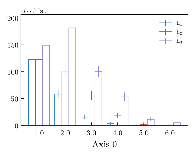
# Create histograms and fill them
h1 = hist.new.Reg(6, 0, 6).Weight().fill(np.random.poisson(0.5, 200))
h2 = hist.new.Reg(6, 0, 6).Weight().fill(np.random.poisson(1.0, 300))
h3 = hist.new.Reg(6, 0, 6).Weight().fill(np.random.poisson(1.2, 500))

fig, ax = plt.subplots()
mh.histplot(
 [h1, h2, h3],
 histtype='bar',
 label=['$h_1$', '$h_2$', '$h_3$'],
 ax=ax
)
mh.cms.label(data=False)
ax.legend(loc='upper right')
mh.yscale_legend(soft_fail=True)
# Optional: move the x-ticks to the bin centers
ax.set_xticks(h1.axes[0].centers)
ax.set_xticklabels([x+0.5 for x in h1.axes[0].centers])
ax.minorticks_off()
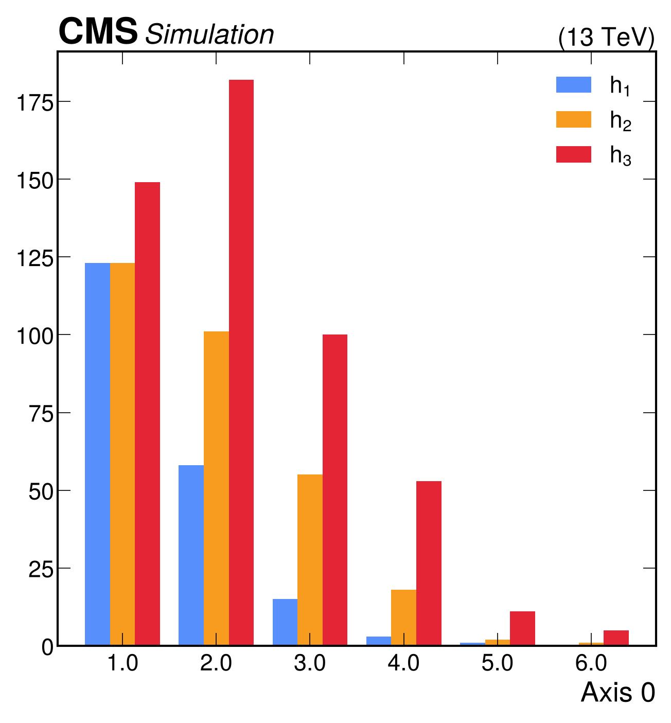
# Create histograms and fill them
h1 = hist.new.Reg(6, 0, 6).Weight().fill(np.random.poisson(0.5, 200))
h2 = hist.new.Reg(6, 0, 6).Weight().fill(np.random.poisson(1.0, 300))
h3 = hist.new.Reg(6, 0, 6).Weight().fill(np.random.poisson(1.2, 500))

fig, ax = plt.subplots()
mh.histplot(
 [h1, h2, h3],
 histtype='barstep',
 label=['$h_1$', '$h_2$', '$h_3$'],
 ax=ax
)
mh.cms.label(data=False)
ax.legend(loc='upper right')
mh.yscale_legend(soft_fail=True)
# Optional: move the x-ticks to the bin centers
ax.set_xticks(h1.axes[0].centers)
ax.set_xticklabels([x+0.5 for x in h1.axes[0].centers])
ax.minorticks_off()
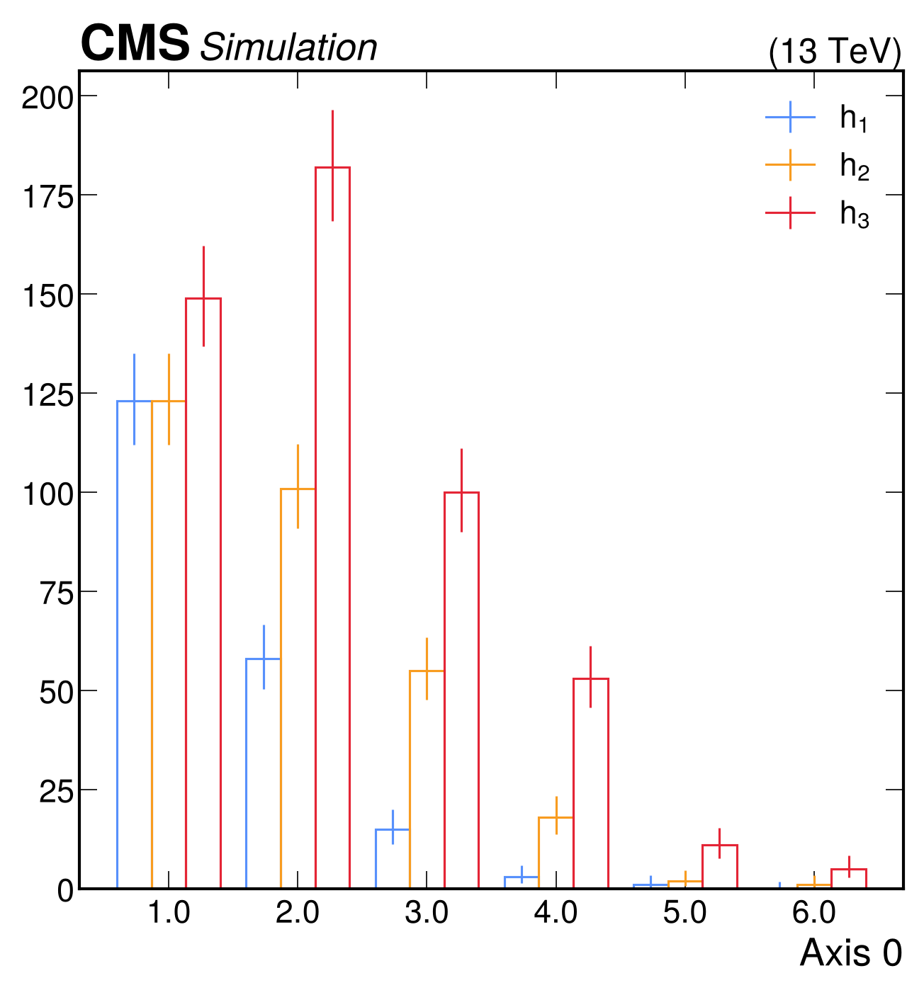
# Create histograms and fill them
h1 = hist.new.Reg(6, 0, 6).Weight().fill(np.random.poisson(0.5, 200))
h2 = hist.new.Reg(6, 0, 6).Weight().fill(np.random.poisson(1.0, 300))
h3 = hist.new.Reg(6, 0, 6).Weight().fill(np.random.poisson(1.2, 500))

fig, ax = plt.subplots()
mh.histplot(
 [h1, h2, h3],
 histtype='bar',
 label=['$h_1$', '$h_2$', '$h_3$'],
 ax=ax
)
mh.atlas.label(data=False)
mh.mpl_magic(soft_fail=True)
ax.legend(loc='upper right')
mh.yscale_legend(soft_fail=True)
# Optional: move the x-ticks to the bin centers
ax.set_xticks(h1.axes[0].centers)
ax.set_xticklabels([x+0.5 for x in h1.axes[0].centers])
ax.minorticks_off()
# Create histograms and fill them
h1 = hist.new.Reg(6, 0, 6).Weight().fill(np.random.poisson(0.5, 200))
h2 = hist.new.Reg(6, 0, 6).Weight().fill(np.random.poisson(1.0, 300))
h3 = hist.new.Reg(6, 0, 6).Weight().fill(np.random.poisson(1.2, 500))

fig, ax = plt.subplots()
mh.histplot(
 [h1, h2, h3],
 histtype='barstep',
 label=['$h_1$', '$h_2$', '$h_3$'],
 ax=ax
)
mh.atlas.label(data=False)
mh.mpl_magic(soft_fail=True)
ax.legend(loc='upper right')
mh.yscale_legend(soft_fail=True)
# Optional: move the x-ticks to the bin centers
ax.set_xticks(h1.axes[0].centers)
ax.set_xticklabels([x+0.5 for x in h1.axes[0].centers])
ax.minorticks_off()
# Create histograms and fill them
h1 = hist.new.Reg(6, 0, 6).Weight().fill(np.random.poisson(0.5, 200))
h2 = hist.new.Reg(6, 0, 6).Weight().fill(np.random.poisson(1.0, 300))
h3 = hist.new.Reg(6, 0, 6).Weight().fill(np.random.poisson(1.2, 500))

fig, ax = plt.subplots()
mh.histplot(
 [h1, h2, h3],
 histtype='bar',
 label=['$h_1$', '$h_2$', '$h_3$'],
 ax=ax
)
mh.lhcb.label(data=False)
ax.legend(loc='upper right')
mh.yscale_legend(soft_fail=True)
# Optional: move the x-ticks to the bin centers
ax.set_xticks(h1.axes[0].centers)
ax.set_xticklabels([x+0.5 for x in h1.axes[0].centers])
ax.minorticks_off()
# Create histograms and fill them
h1 = hist.new.Reg(6, 0, 6).Weight().fill(np.random.poisson(0.5, 200))
h2 = hist.new.Reg(6, 0, 6).Weight().fill(np.random.poisson(1.0, 300))
h3 = hist.new.Reg(6, 0, 6).Weight().fill(np.random.poisson(1.2, 500))

fig, ax = plt.subplots()
mh.histplot(
 [h1, h2, h3],
 histtype='barstep',
 label=['$h_1$', '$h_2$', '$h_3$'],
 ax=ax
)
mh.lhcb.label(data=False)
ax.legend(loc='upper right')
mh.yscale_legend(soft_fail=True)
# Optional: move the x-ticks to the bin centers
ax.set_xticks(h1.axes[0].centers)
ax.set_xticklabels([x+0.5 for x in h1.axes[0].centers])
ax.minorticks_off()
# Create histograms and fill them
h1 = hist.new.Reg(6, 0, 6).Weight().fill(np.random.poisson(0.5, 200))
h2 = hist.new.Reg(6, 0, 6).Weight().fill(np.random.poisson(1.0, 300))
h3 = hist.new.Reg(6, 0, 6).Weight().fill(np.random.poisson(1.2, 500))

fig, ax = plt.subplots()
mh.histplot(
 [h1, h2, h3],
 histtype='bar',
 label=['$h_1$', '$h_2$', '$h_3$'],
 ax=ax
)
mh.alice.label(data=False)
mh.mpl_magic(soft_fail=True)
ax.legend(loc='upper right')
mh.yscale_legend(soft_fail=True)
# Optional: move the x-ticks to the bin centers
ax.set_xticks(h1.axes[0].centers)
ax.set_xticklabels([x+0.5 for x in h1.axes[0].centers])
ax.minorticks_off()
# Create histograms and fill them
h1 = hist.new.Reg(6, 0, 6).Weight().fill(np.random.poisson(0.5, 200))
h2 = hist.new.Reg(6, 0, 6).Weight().fill(np.random.poisson(1.0, 300))
h3 = hist.new.Reg(6, 0, 6).Weight().fill(np.random.poisson(1.2, 500))

fig, ax = plt.subplots()
mh.histplot(
 [h1, h2, h3],
 histtype='barstep',
 label=['$h_1$', '$h_2$', '$h_3$'],
 ax=ax
)
mh.alice.label(data=False)
mh.mpl_magic(soft_fail=True)
ax.legend(loc='upper right')
mh.yscale_legend(soft_fail=True)
# Optional: move the x-ticks to the bin centers
ax.set_xticks(h1.axes[0].centers)
ax.set_xticklabels([x+0.5 for x in h1.axes[0].centers])
ax.minorticks_off()
# Create histograms and fill them
h1 = hist.new.Reg(6, 0, 6).Weight().fill(np.random.poisson(0.5, 200))
h2 = hist.new.Reg(6, 0, 6).Weight().fill(np.random.poisson(1.0, 300))
h3 = hist.new.Reg(6, 0, 6).Weight().fill(np.random.poisson(1.2, 500))

fig, ax = plt.subplots()
mh.histplot(
 [h1, h2, h3],
 histtype='bar',
 label=['$h_1$', '$h_2$', '$h_3$'],
 ax=ax
)
mh.dune.label(data=False)
ax.legend(loc='upper right')
mh.yscale_legend(soft_fail=True)
# Optional: move the x-ticks to the bin centers
ax.set_xticks(h1.axes[0].centers)
ax.set_xticklabels([x+0.5 for x in h1.axes[0].centers])
ax.minorticks_off()
# Create histograms and fill them
h1 = hist.new.Reg(6, 0, 6).Weight().fill(np.random.poisson(0.5, 200))
h2 = hist.new.Reg(6, 0, 6).Weight().fill(np.random.poisson(1.0, 300))
h3 = hist.new.Reg(6, 0, 6).Weight().fill(np.random.poisson(1.2, 500))

fig, ax = plt.subplots()
mh.histplot(
 [h1, h2, h3],
 histtype='barstep',
 label=['$h_1$', '$h_2$', '$h_3$'],
 ax=ax
)
mh.dune.label(data=False)
ax.legend(loc='upper right')
mh.yscale_legend(soft_fail=True)
# Optional: move the x-ticks to the bin centers
ax.set_xticks(h1.axes[0].centers)
ax.set_xticklabels([x+0.5 for x in h1.axes[0].centers])
ax.minorticks_off()
Blinding¤
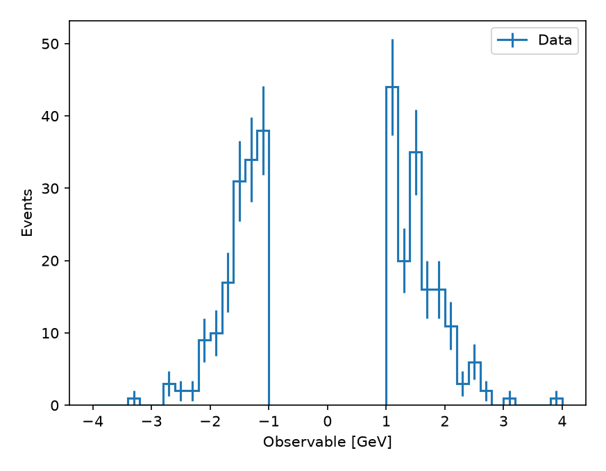
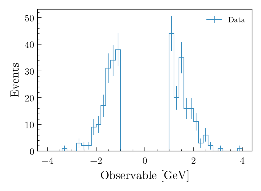
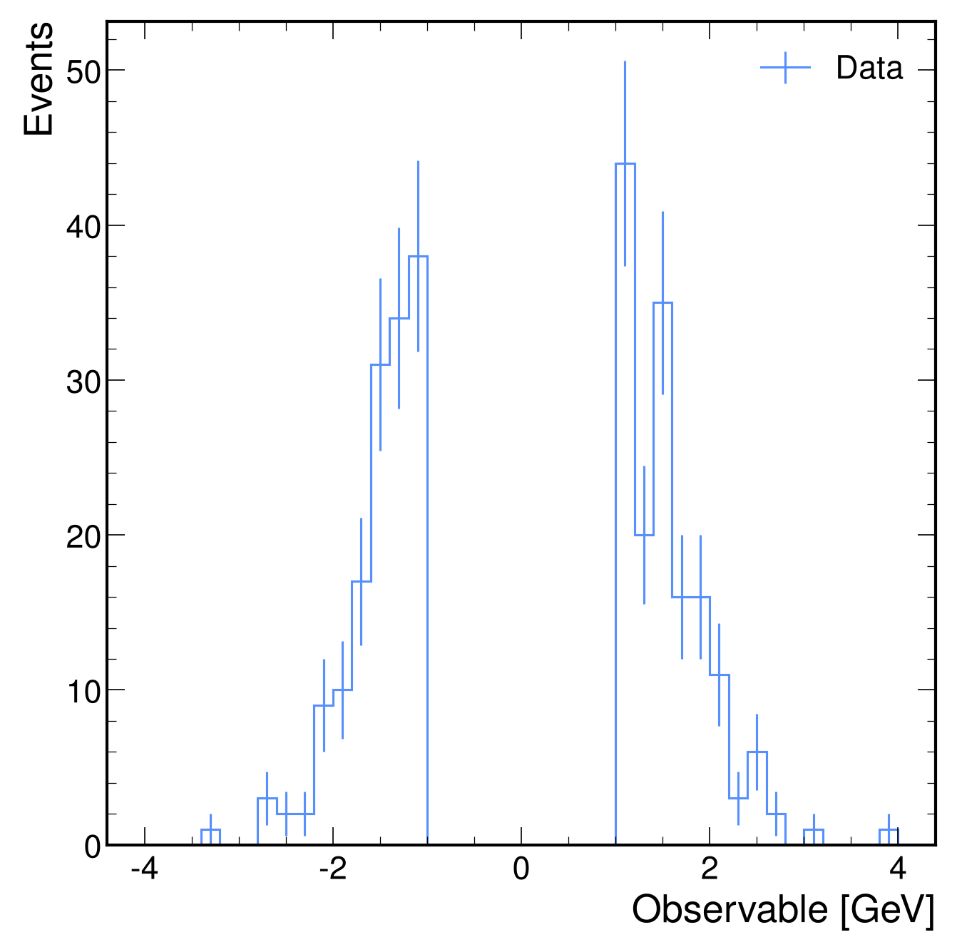
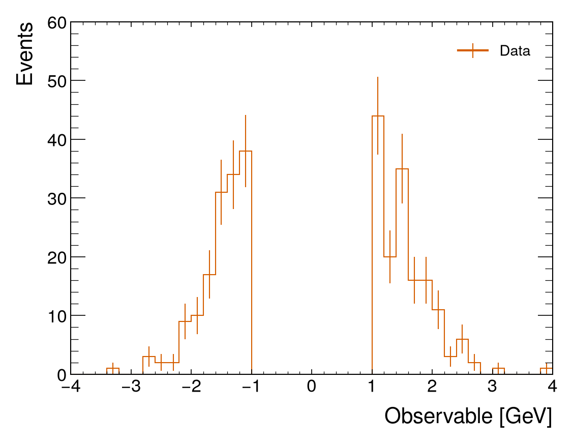
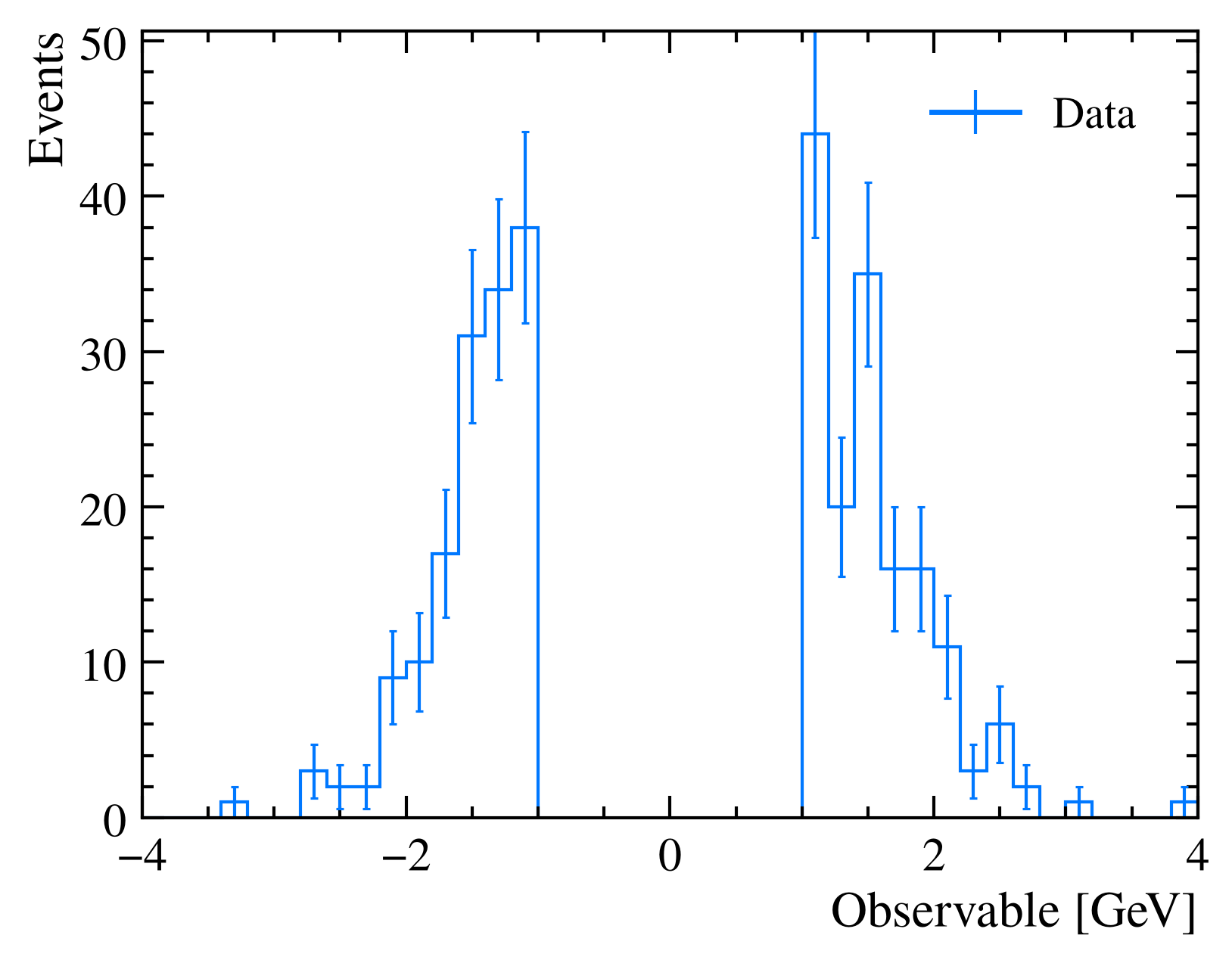
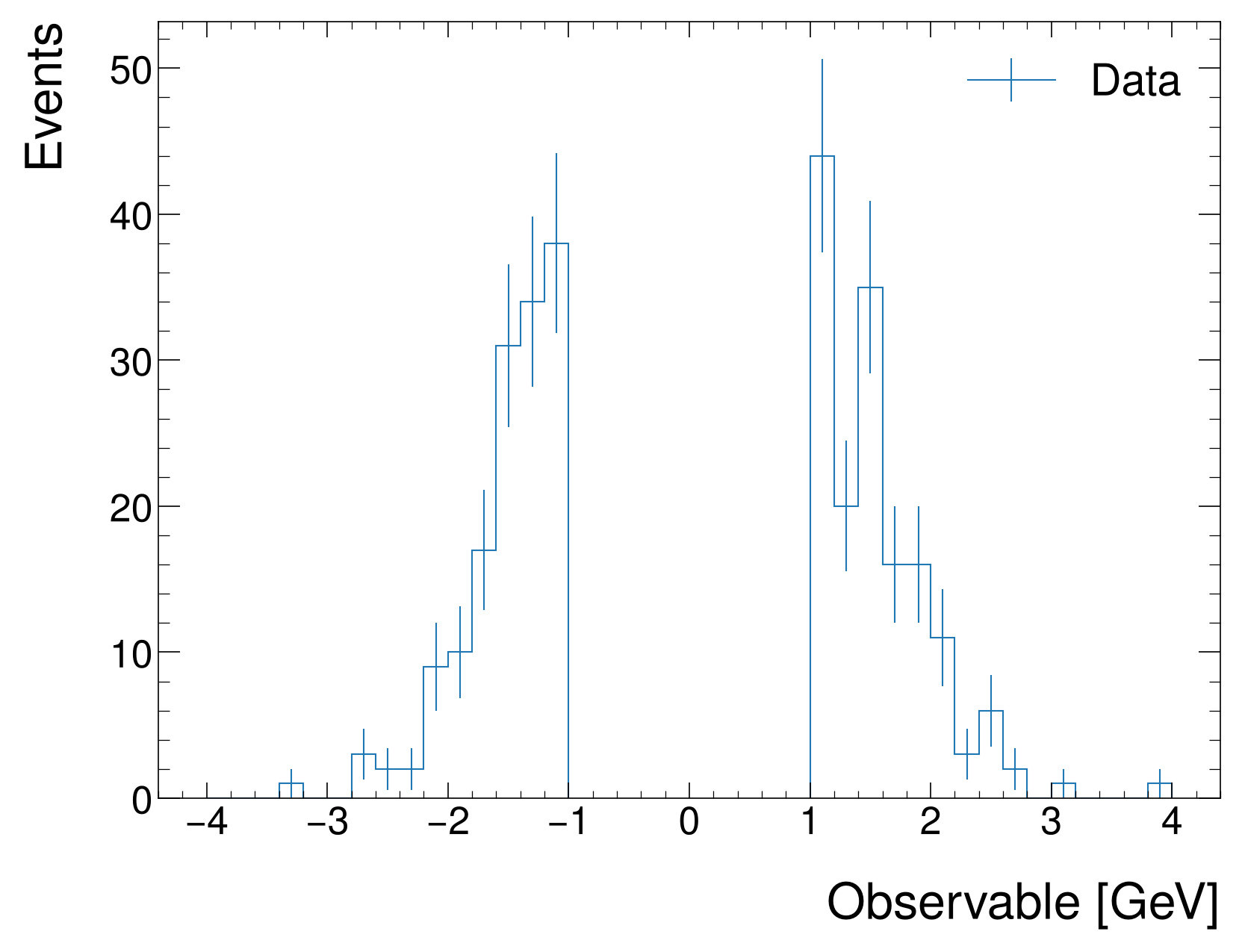
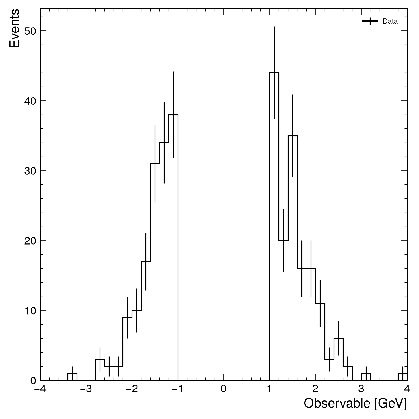
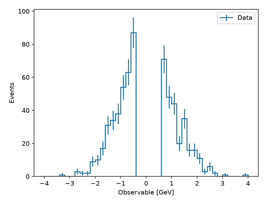
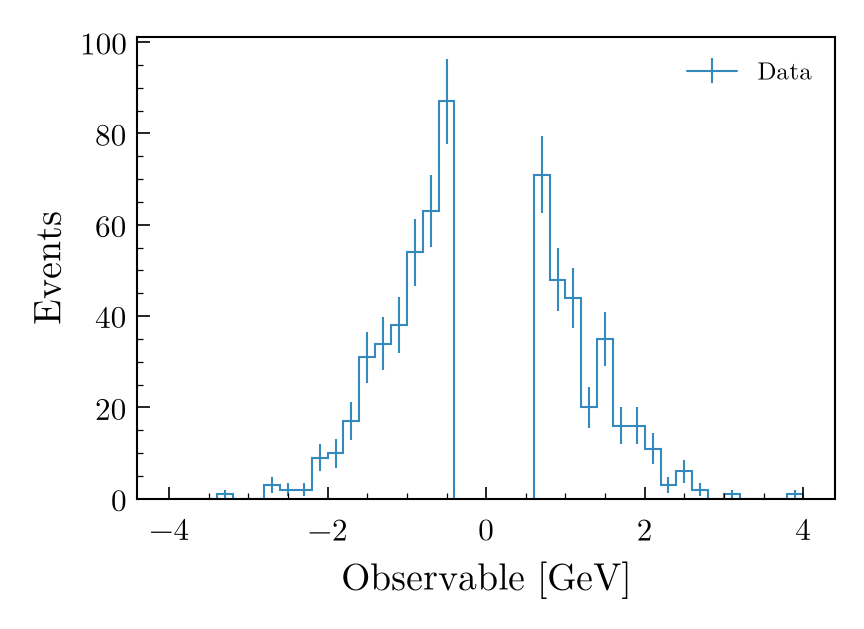
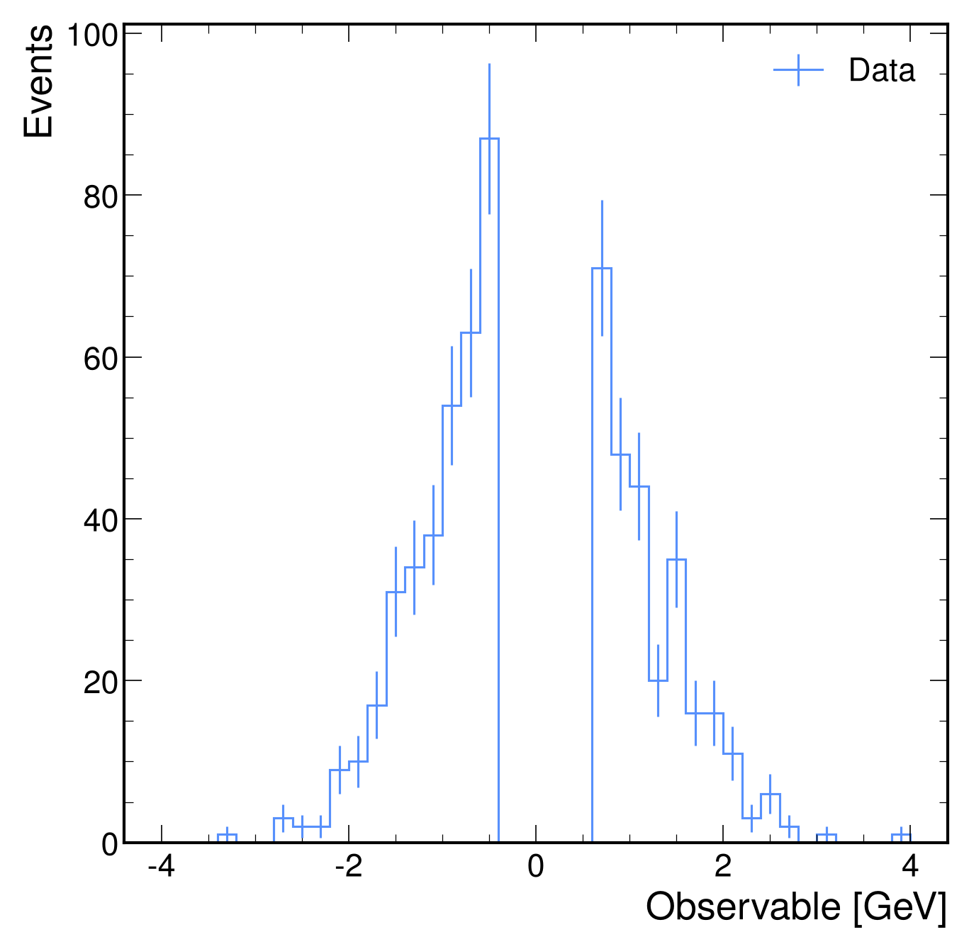
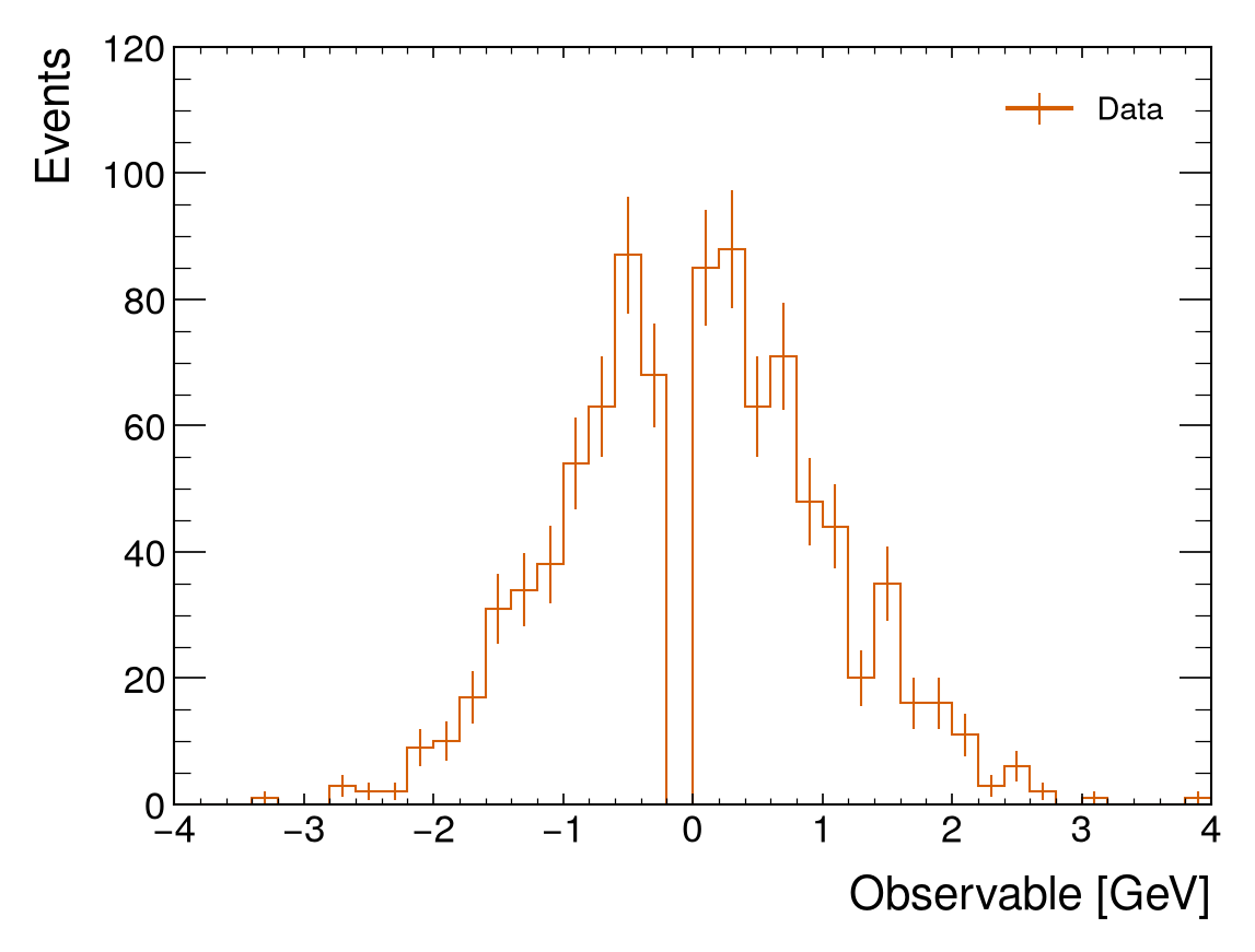
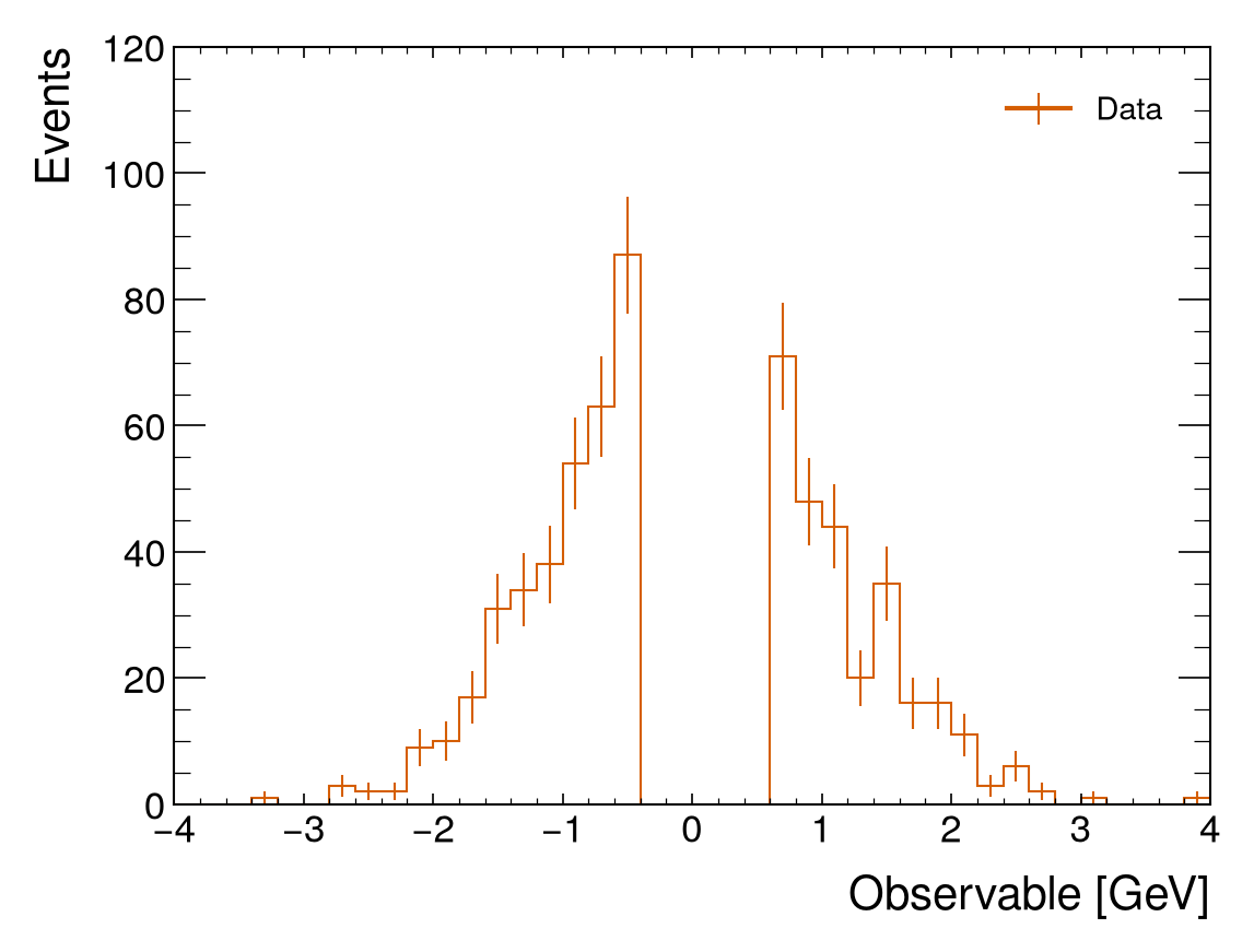
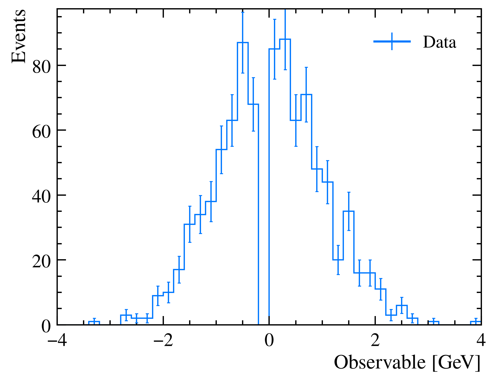
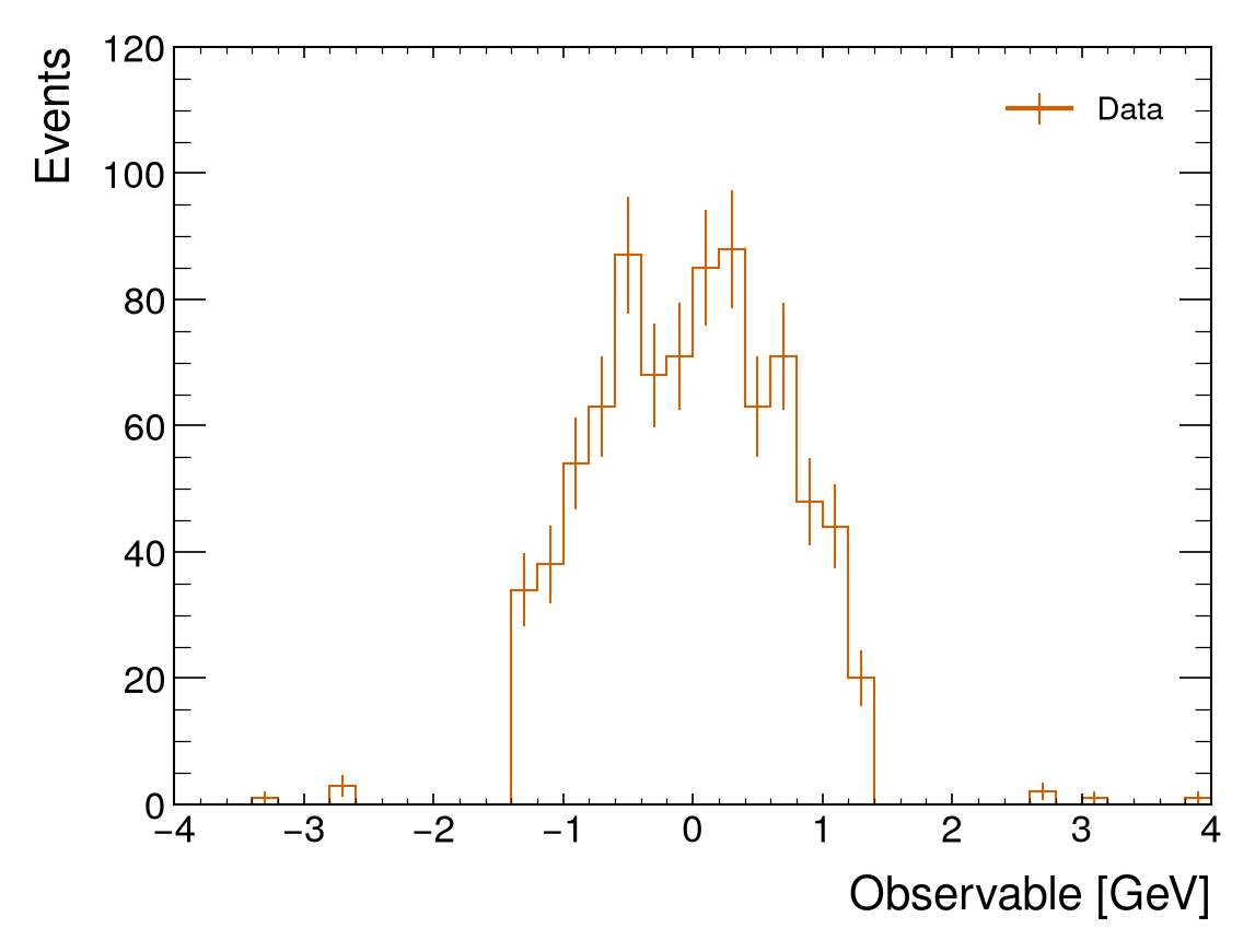
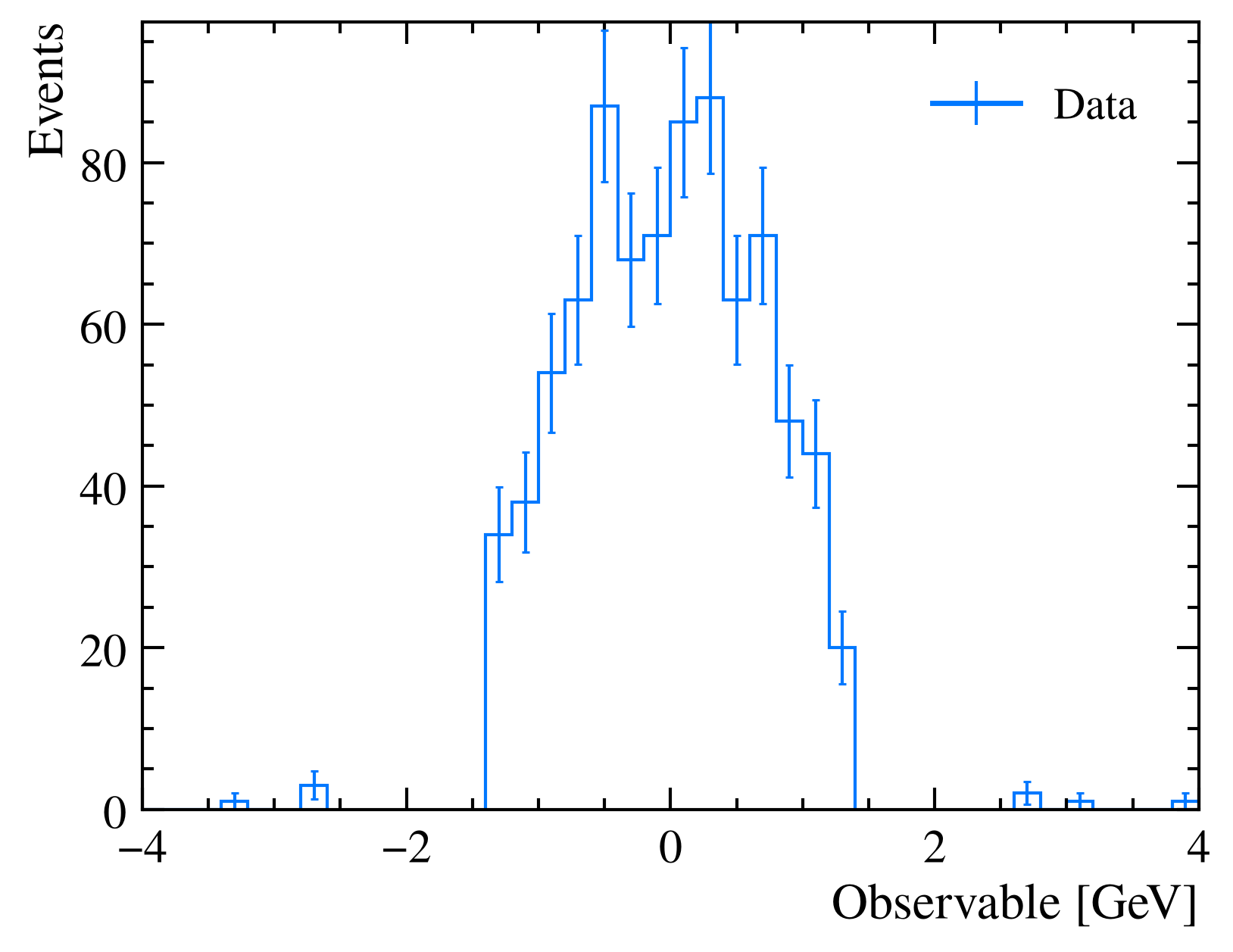
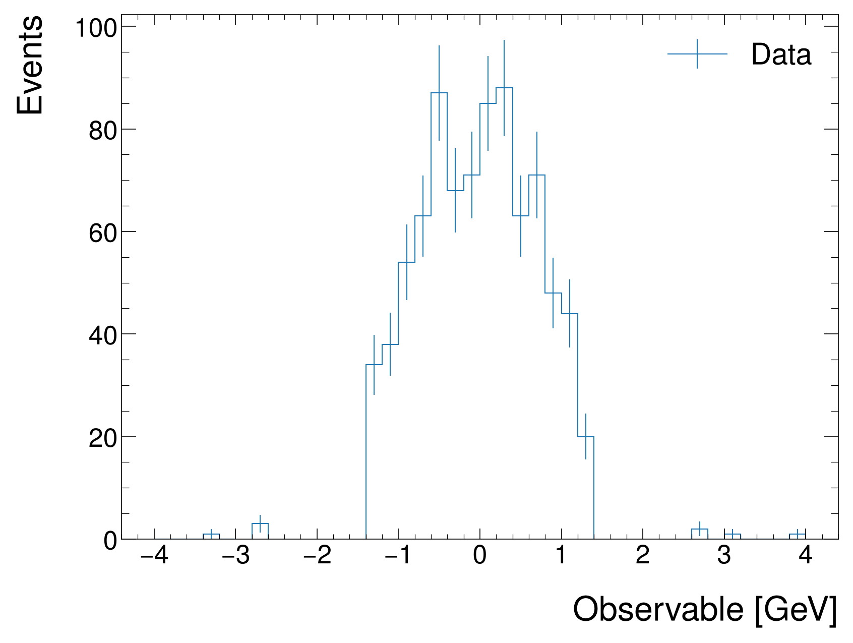
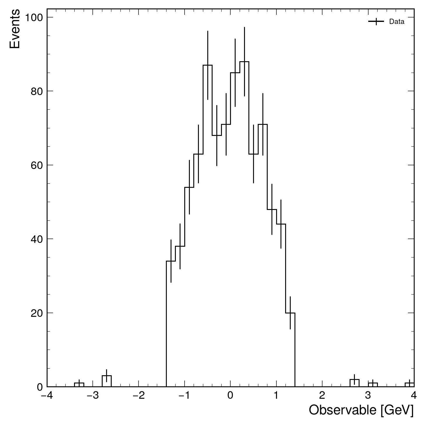
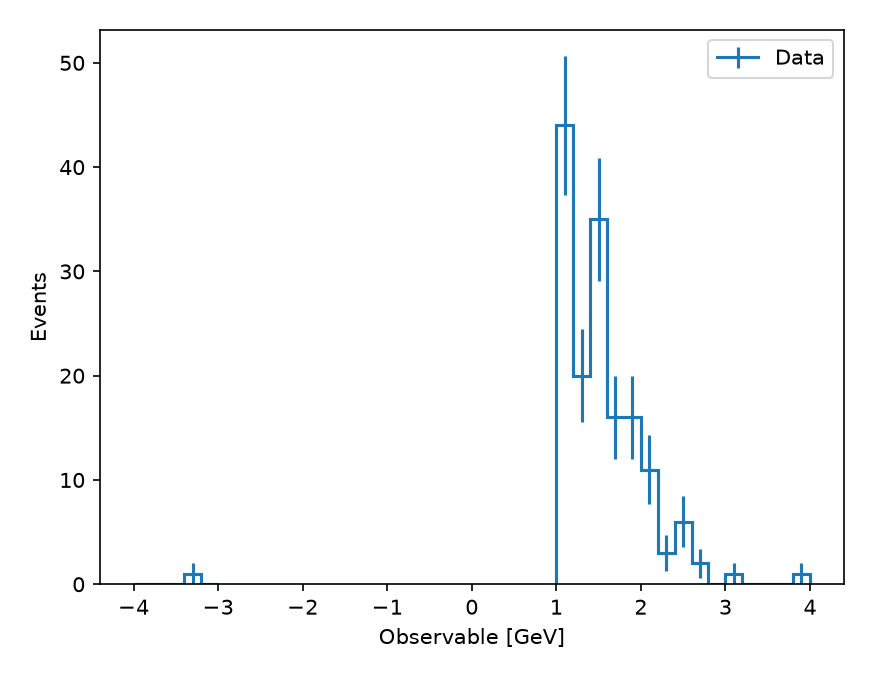
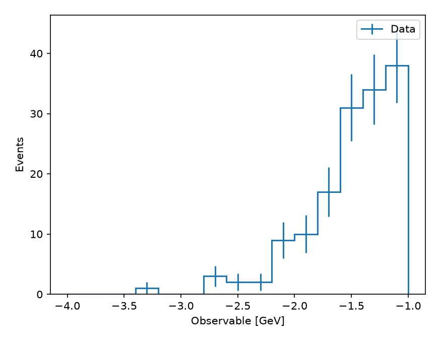
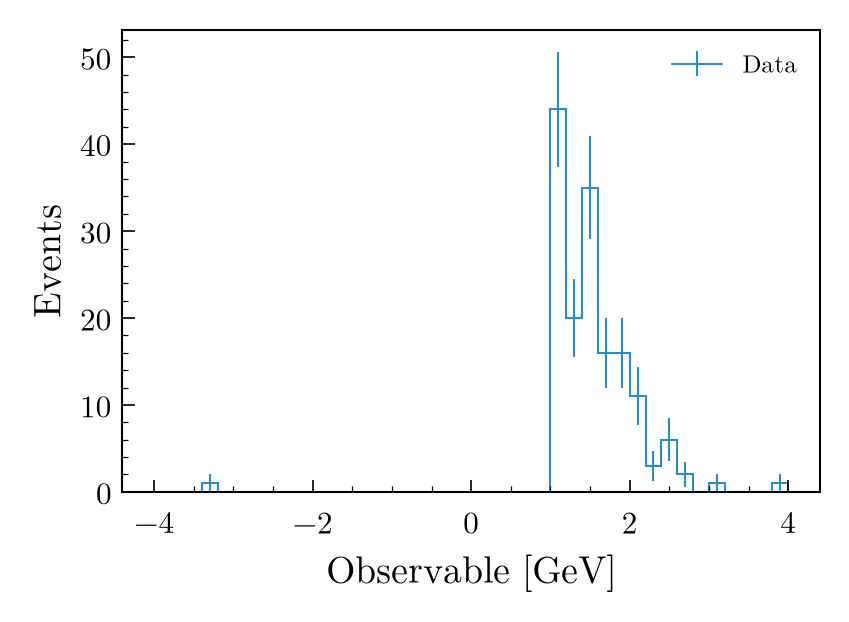
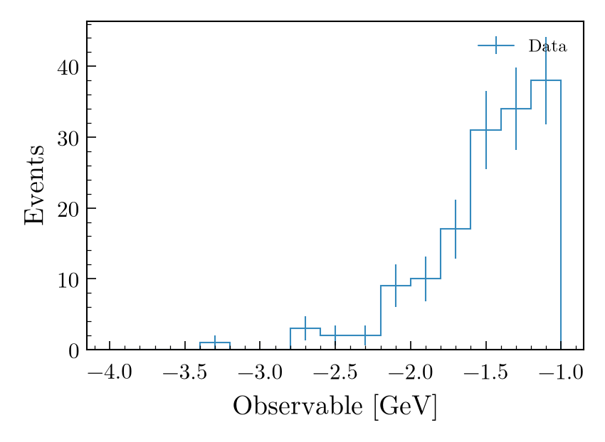
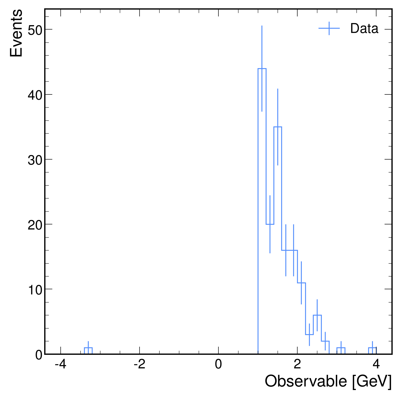
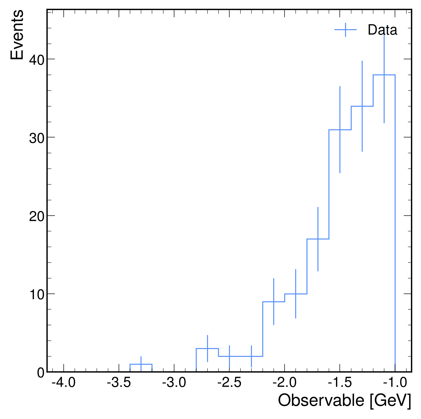
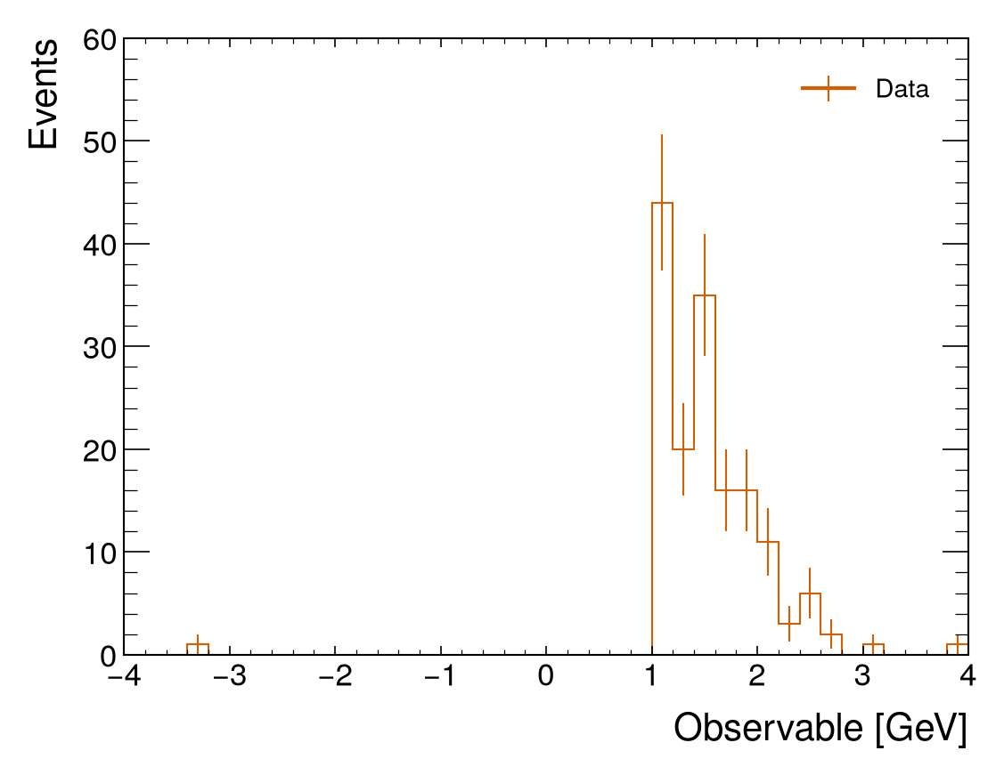
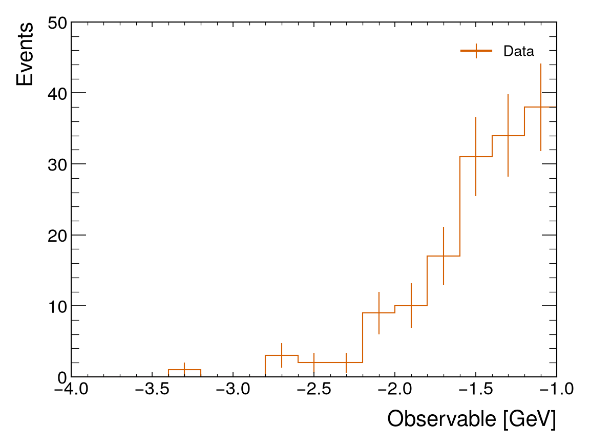
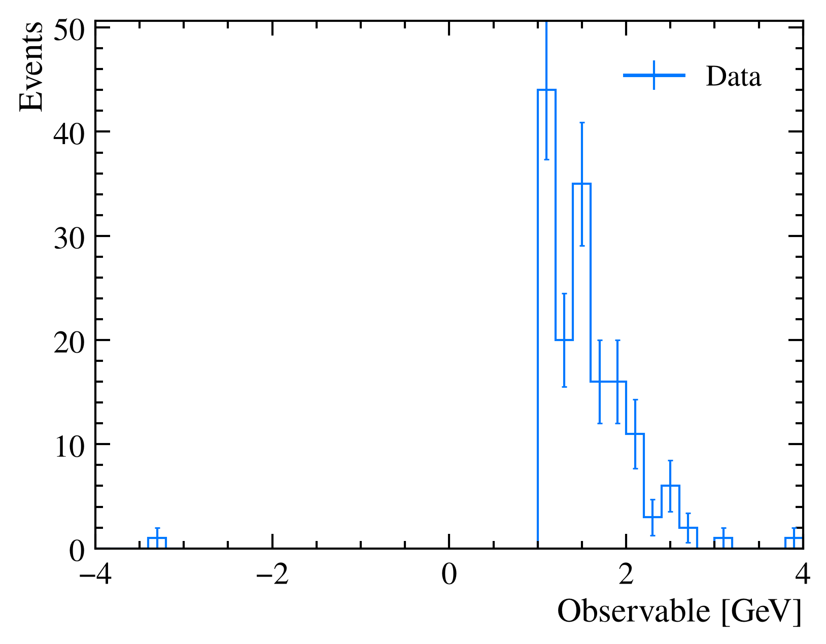
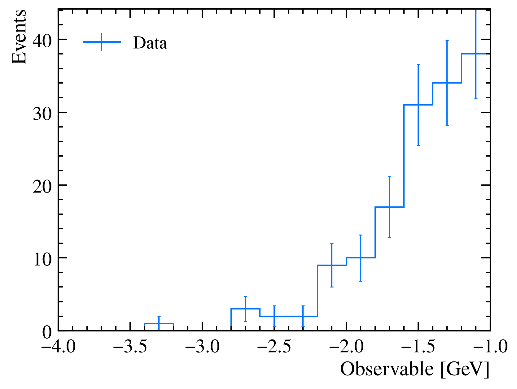
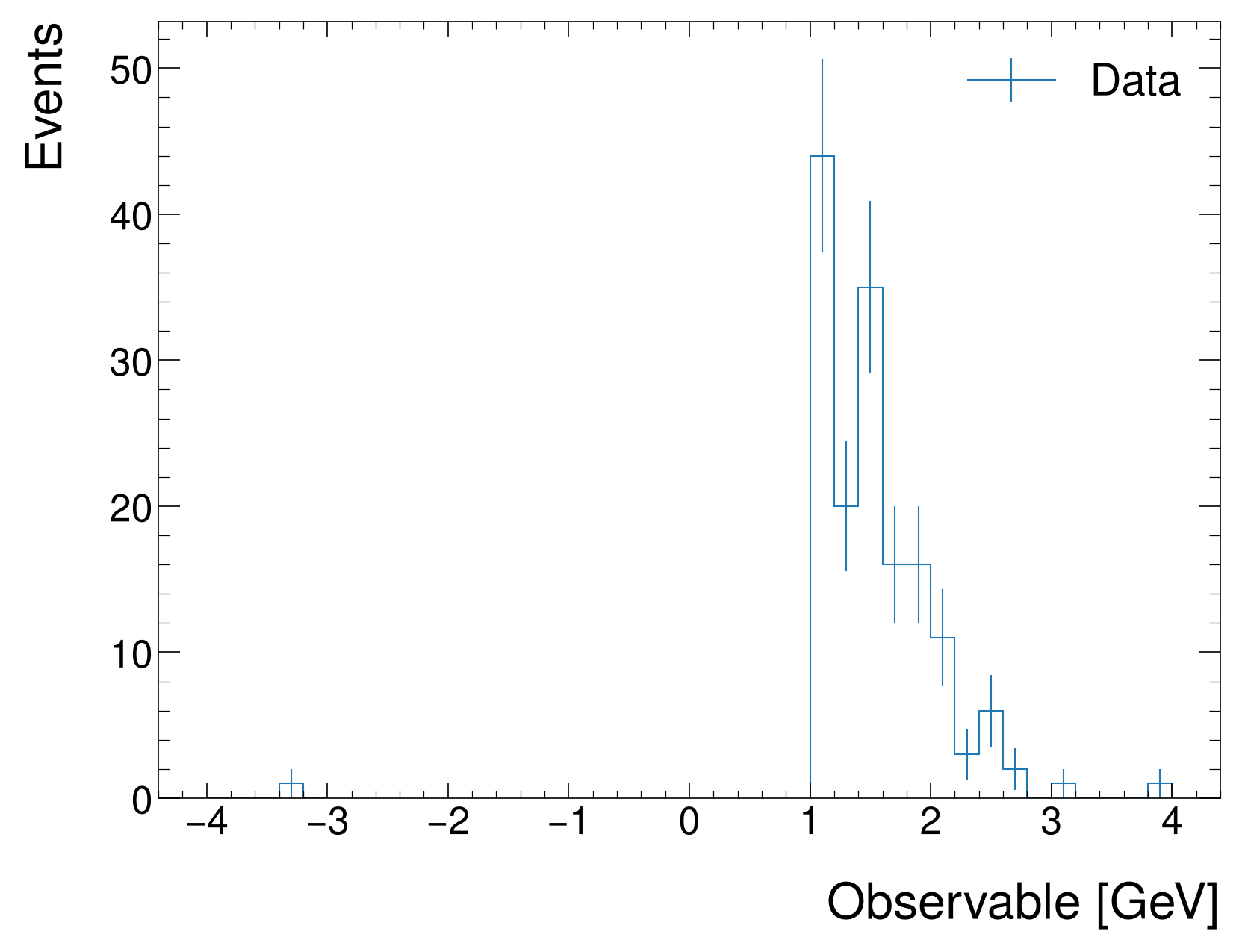
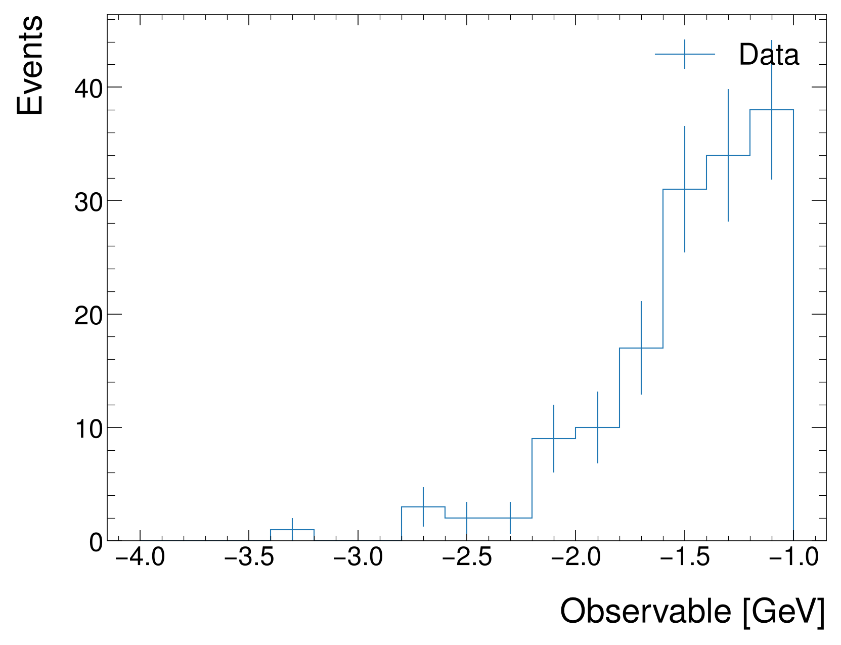
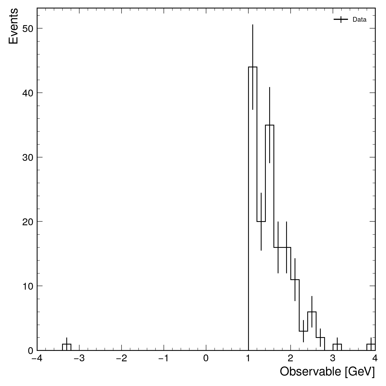
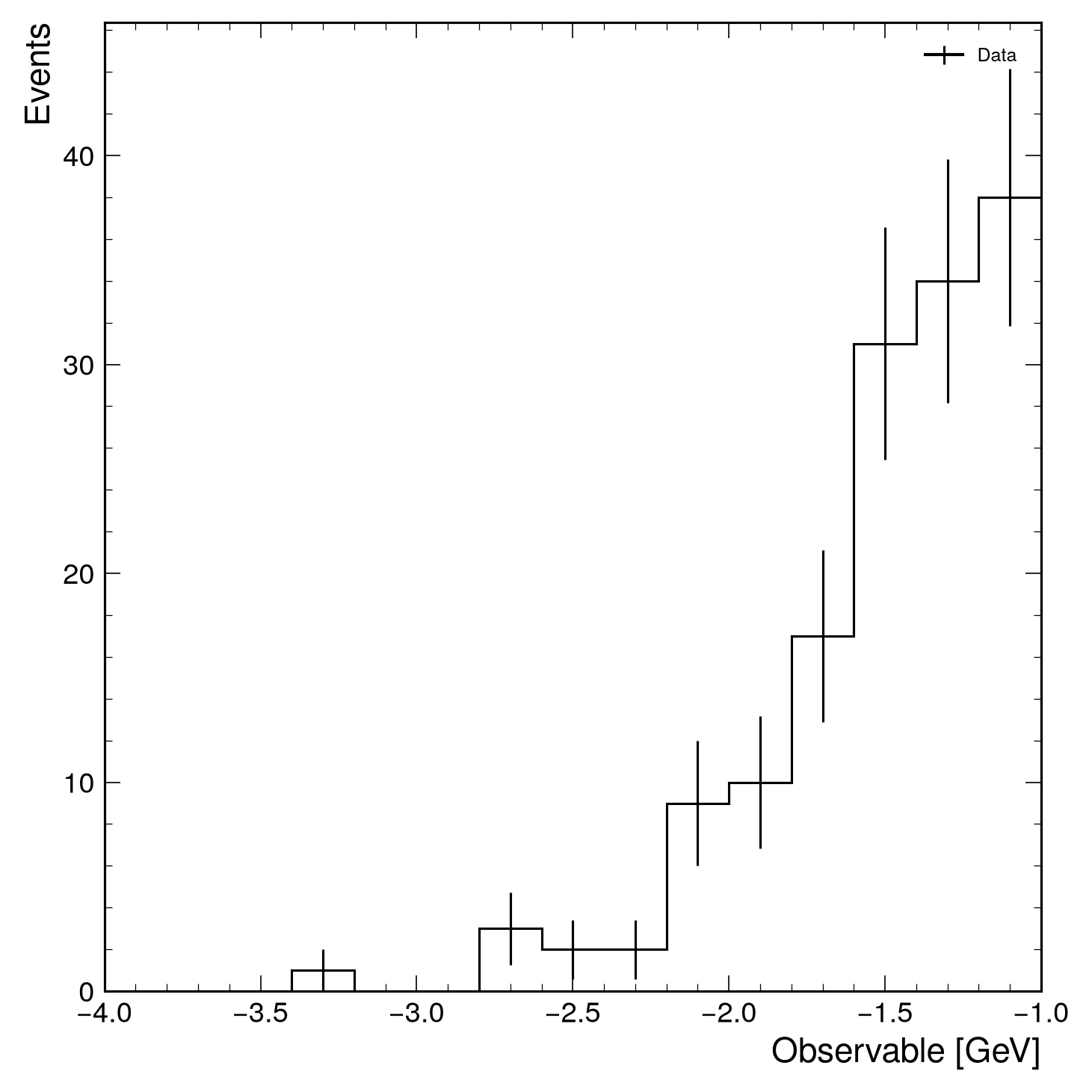
Blinding allows you to hide specific regions of a histogram, which is useful for blind analyses where signal regions should not be examined until the analysis is finalized. The blind parameter in mh.histplot() supports multiple specification formats to accommodate different use cases.
Blinding syntax overview
Blinding regions can be specified in several ways:
- Value-based: Specify physical values (coordinates) using tuples or
jsuffix - Index-based: Specify bin indices directly using integers
- Multiple regions: Use a list to blind multiple regions at once
All formats can be combined in a list for maximum flexibility.
Value-Based Blinding¤
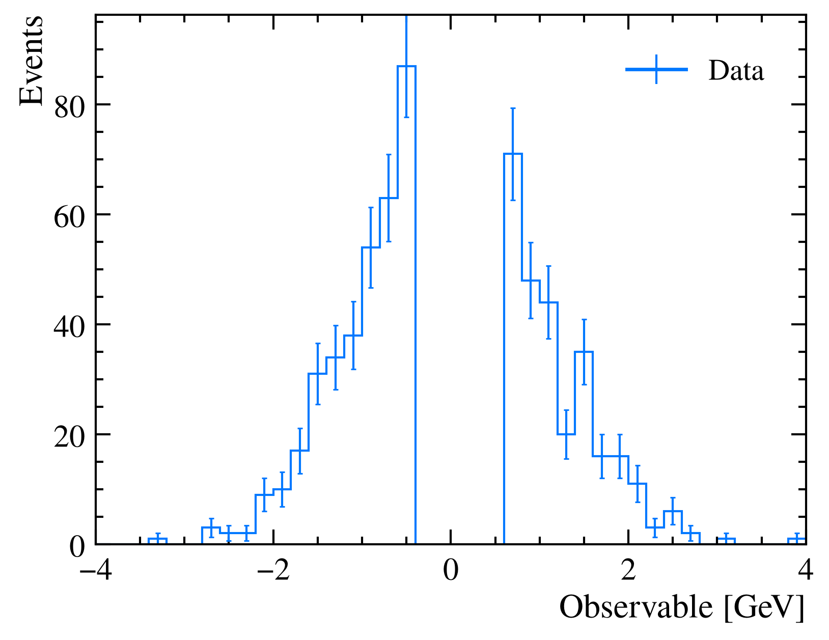
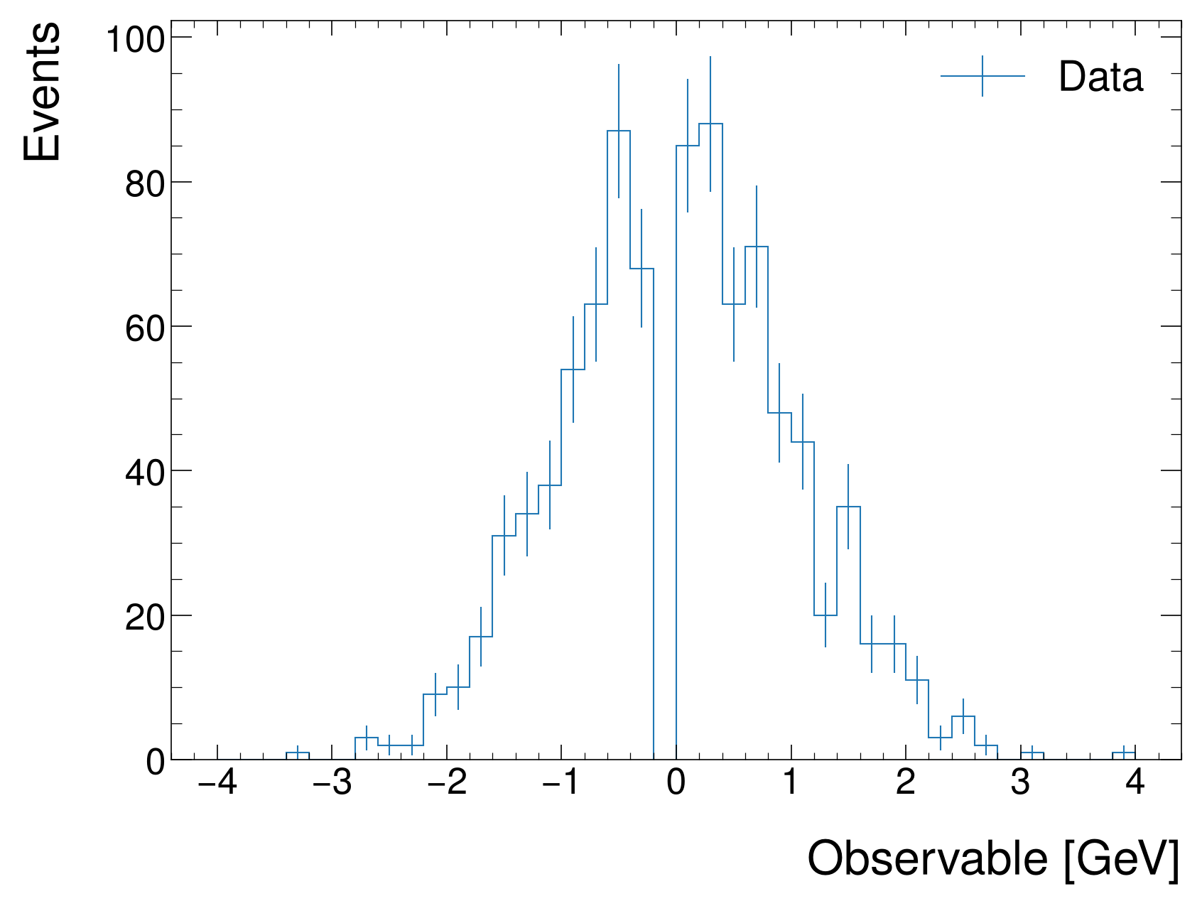
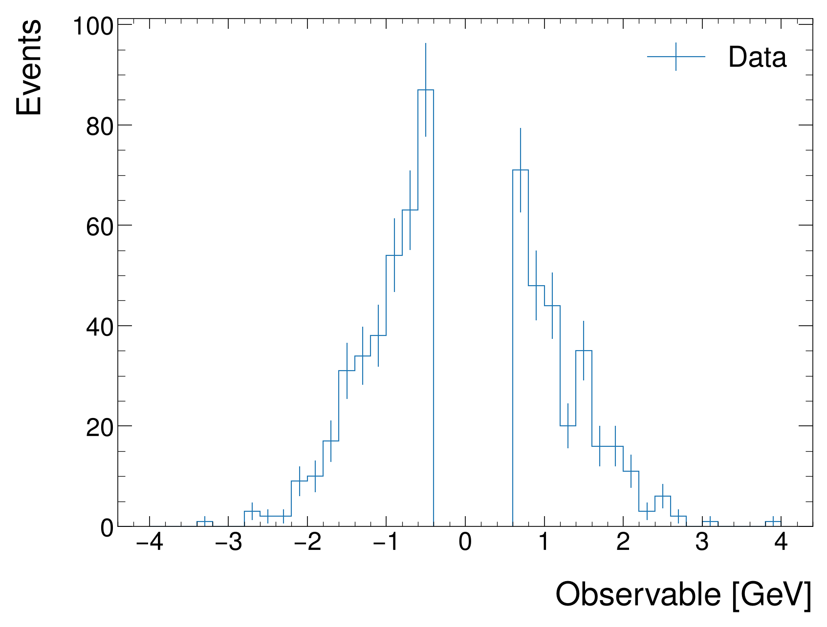
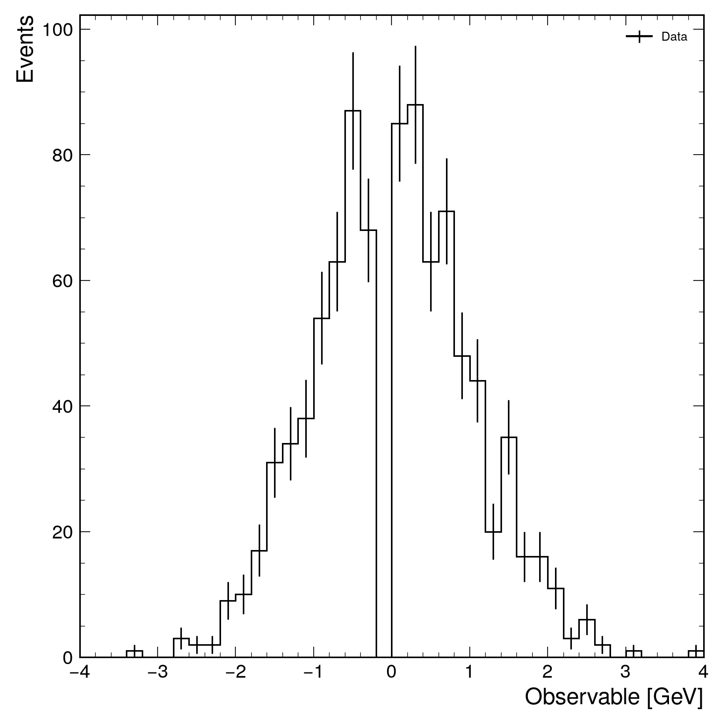
Blind a region by specifying physical values (coordinates) on the x-axis:
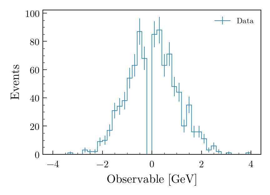
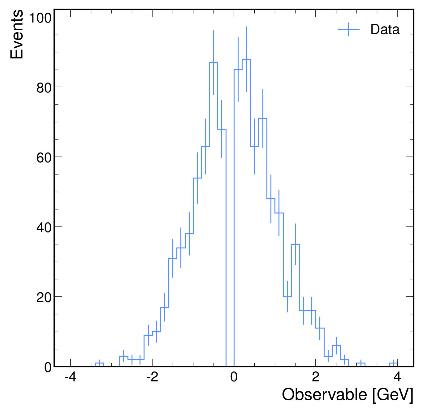
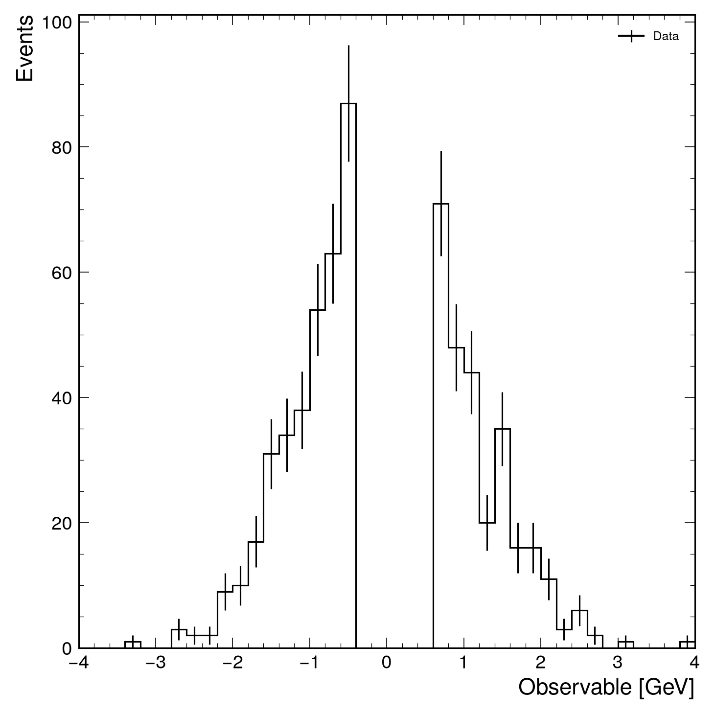
Index-Based Blinding¤
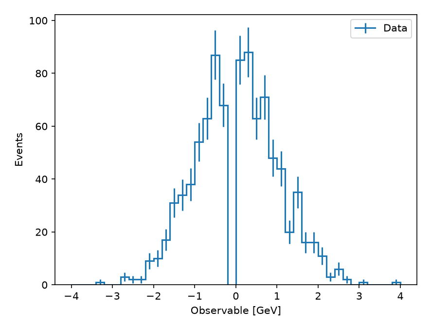
Blind specific bins by their index:
Multiple Regions¤
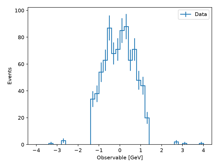
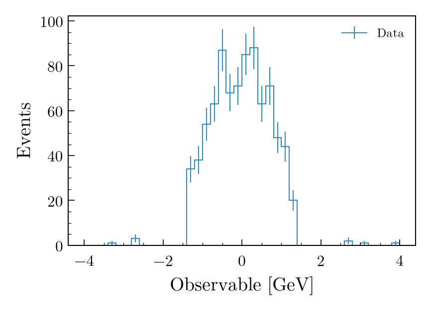
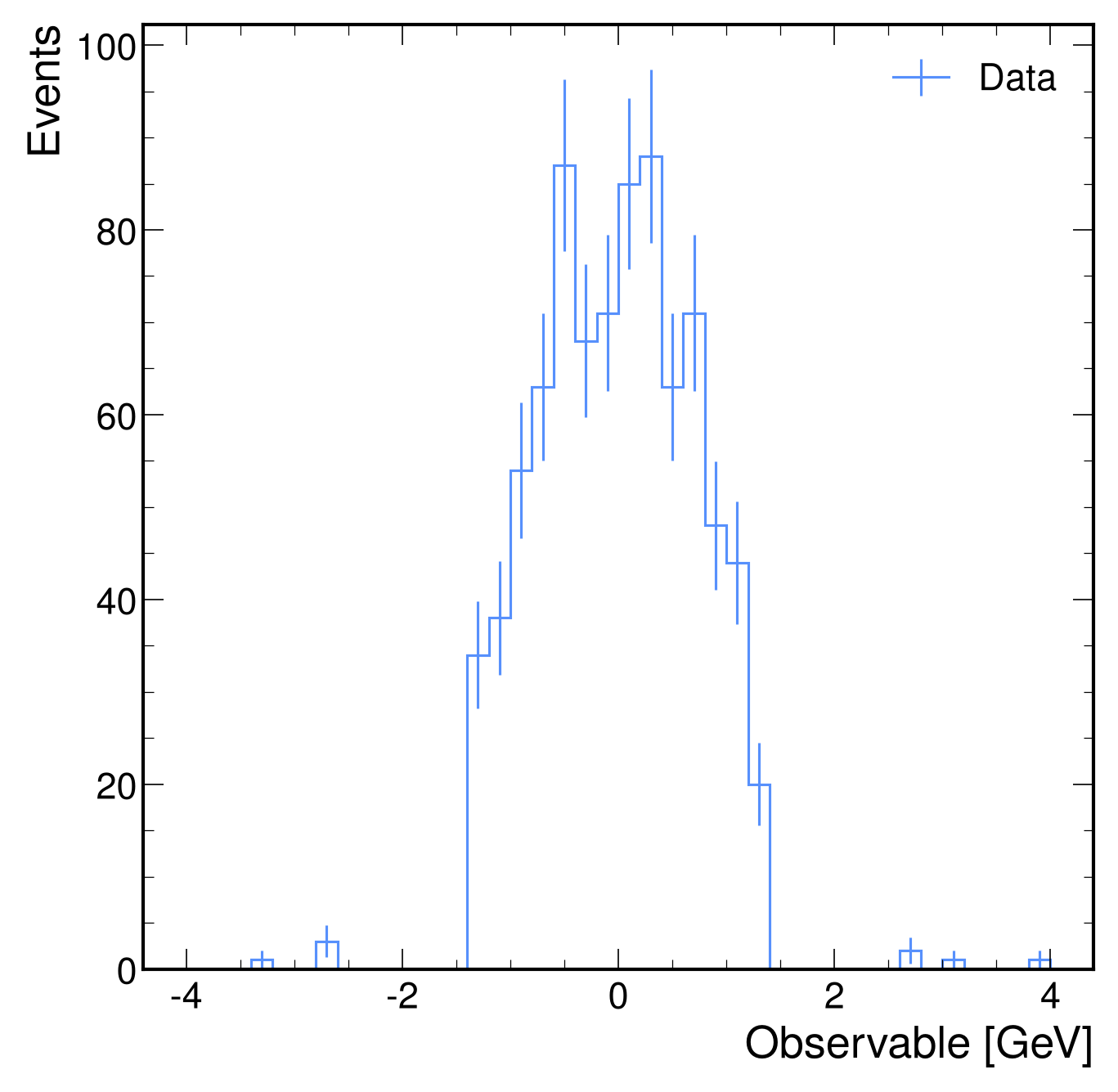
Blind multiple regions by providing a list of specifications:
Mixed-Mode Blinding¤
Mix value-based and index-based specifications in the same slice:
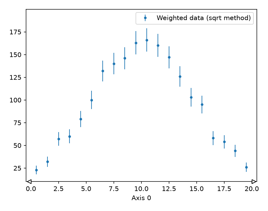
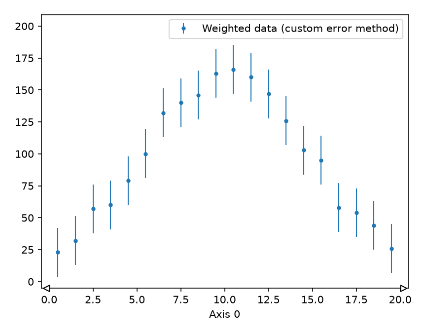
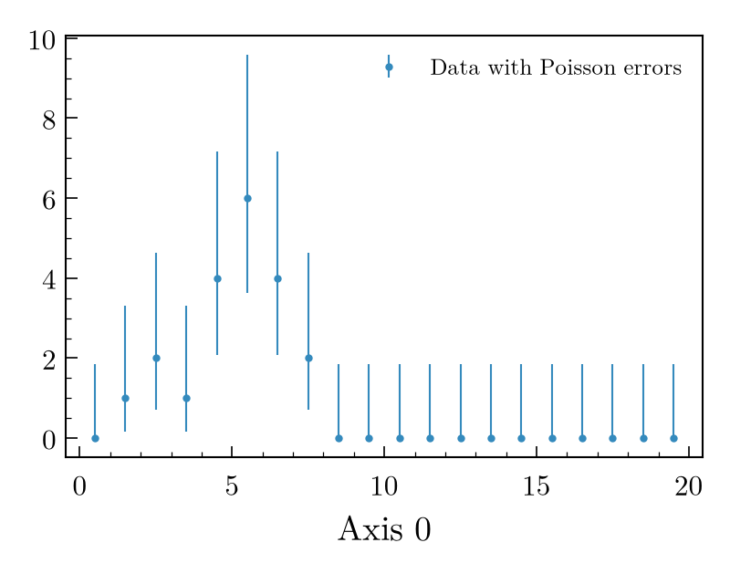
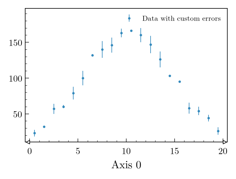
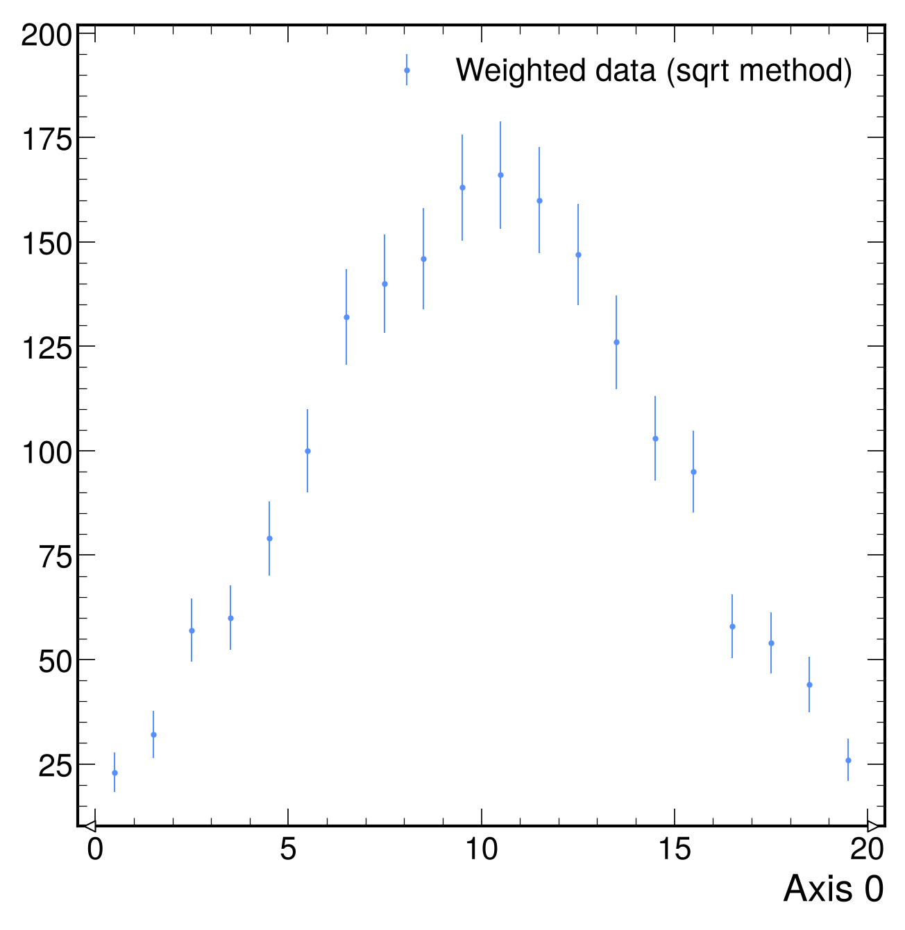
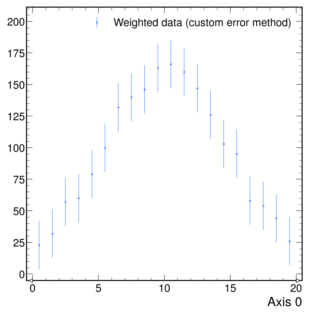
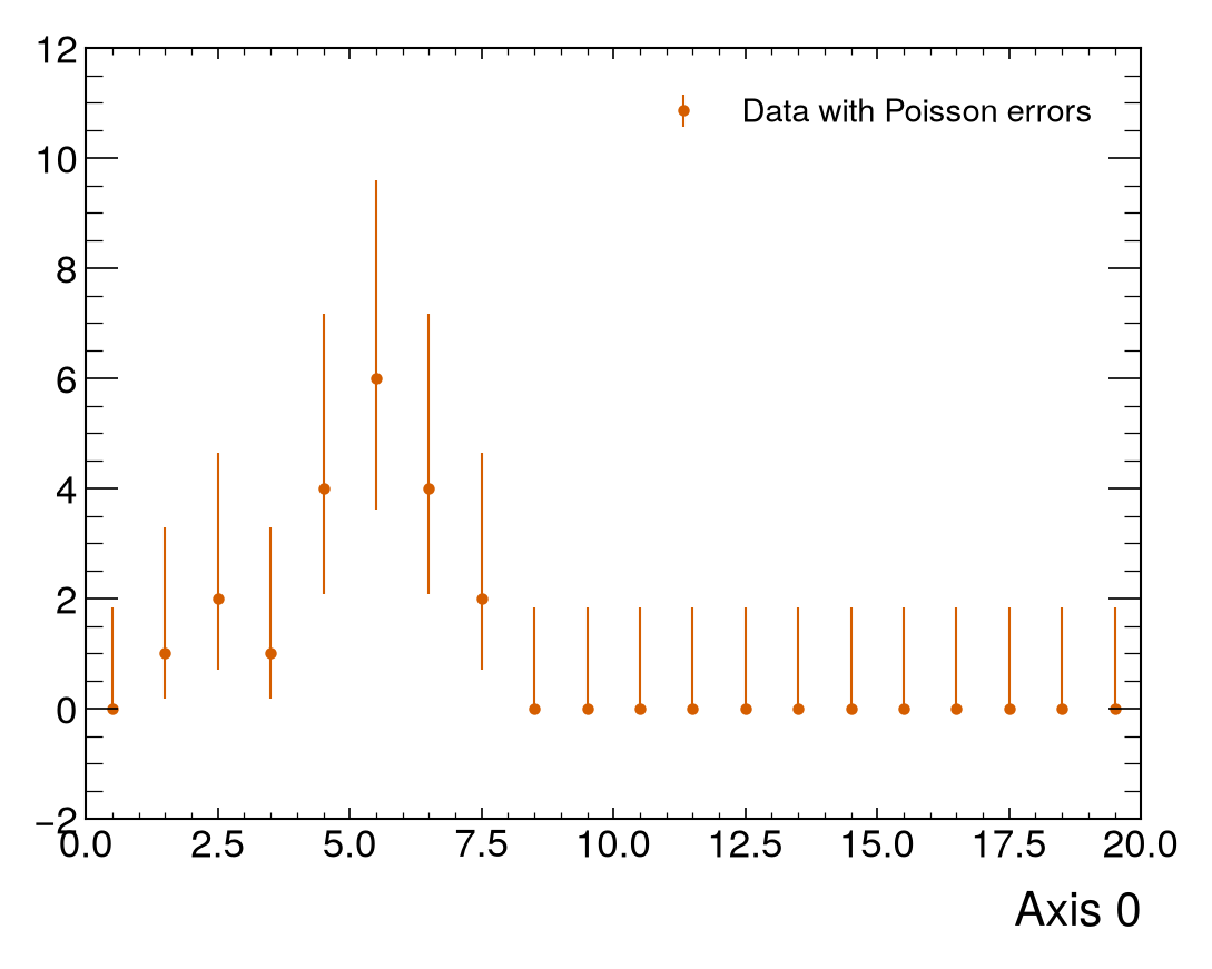
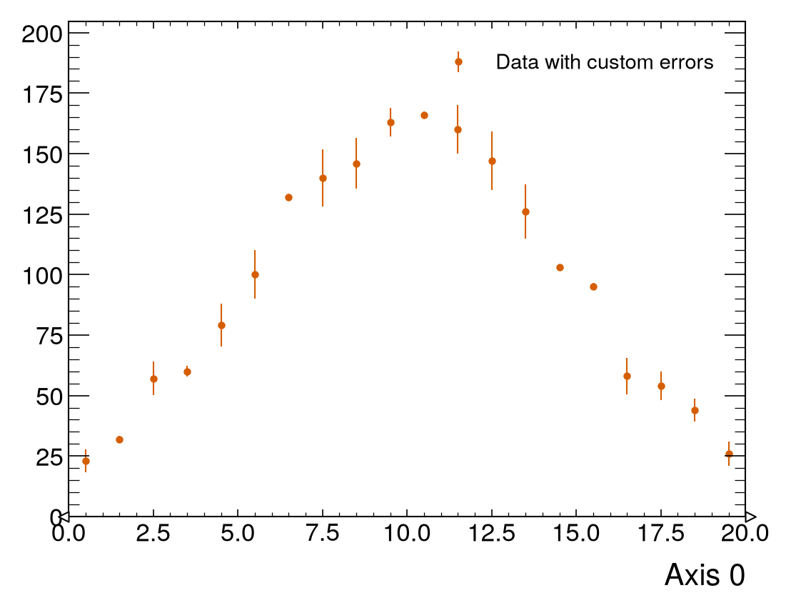
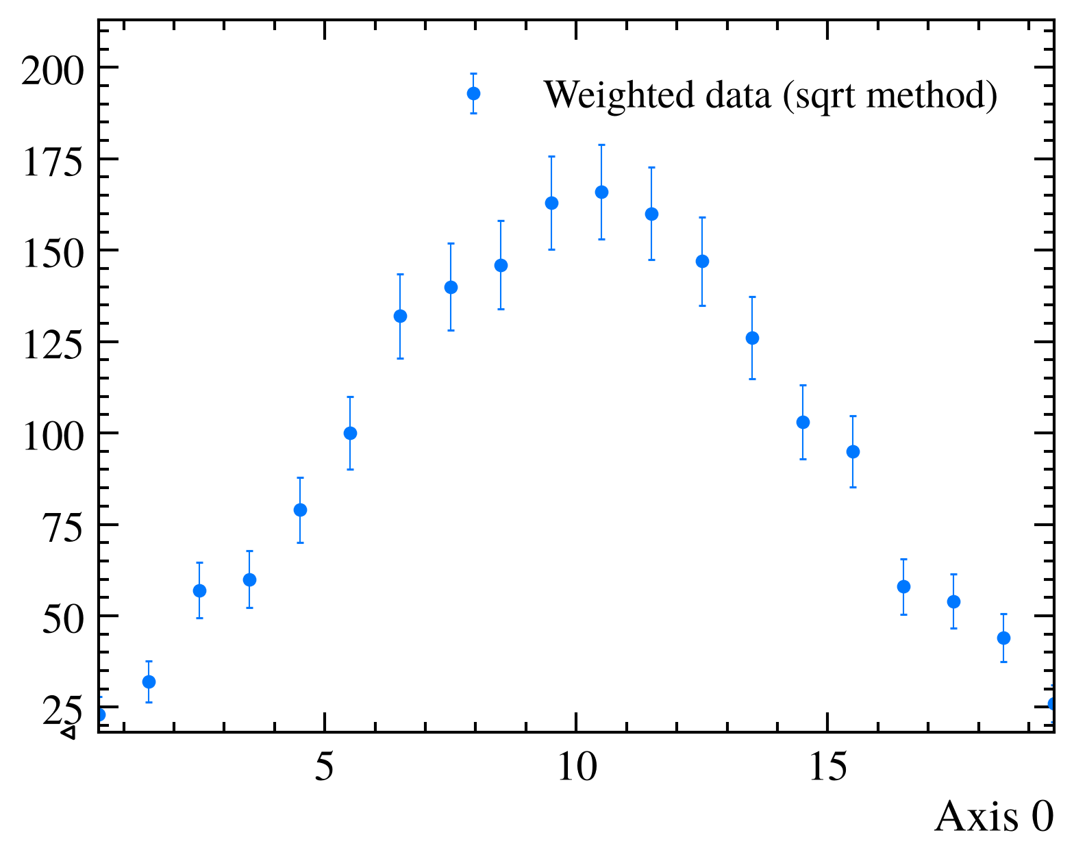
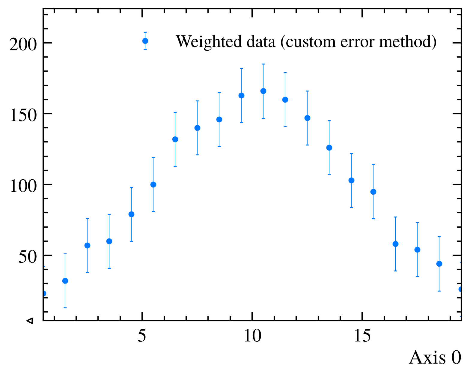
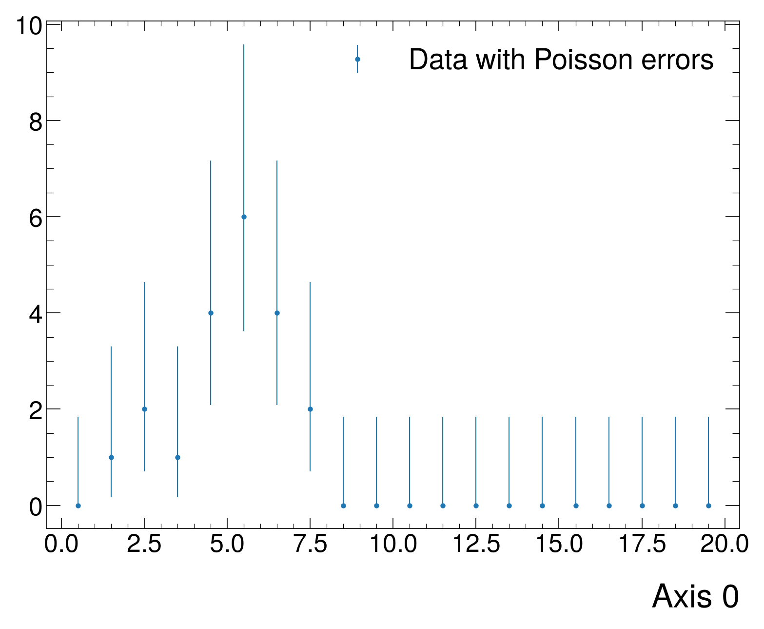
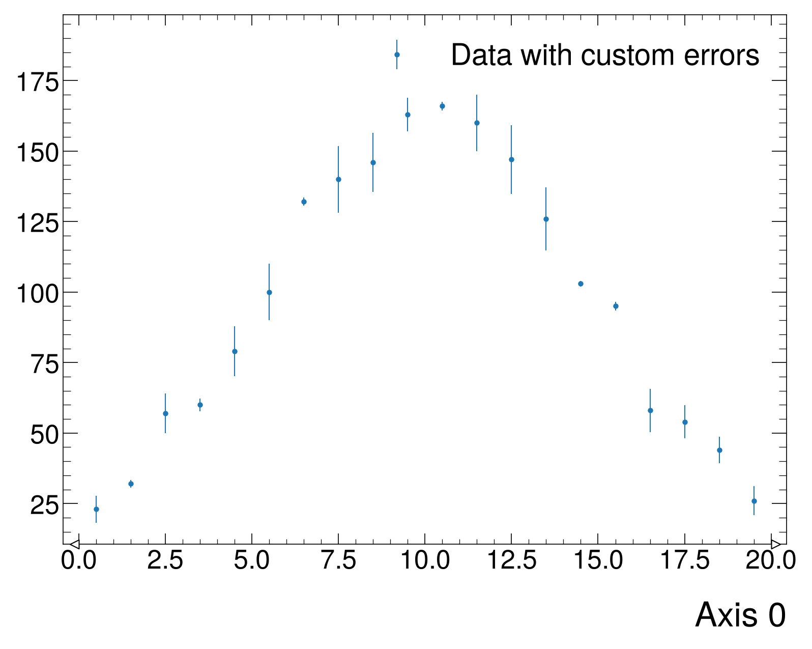
Error Bars¤
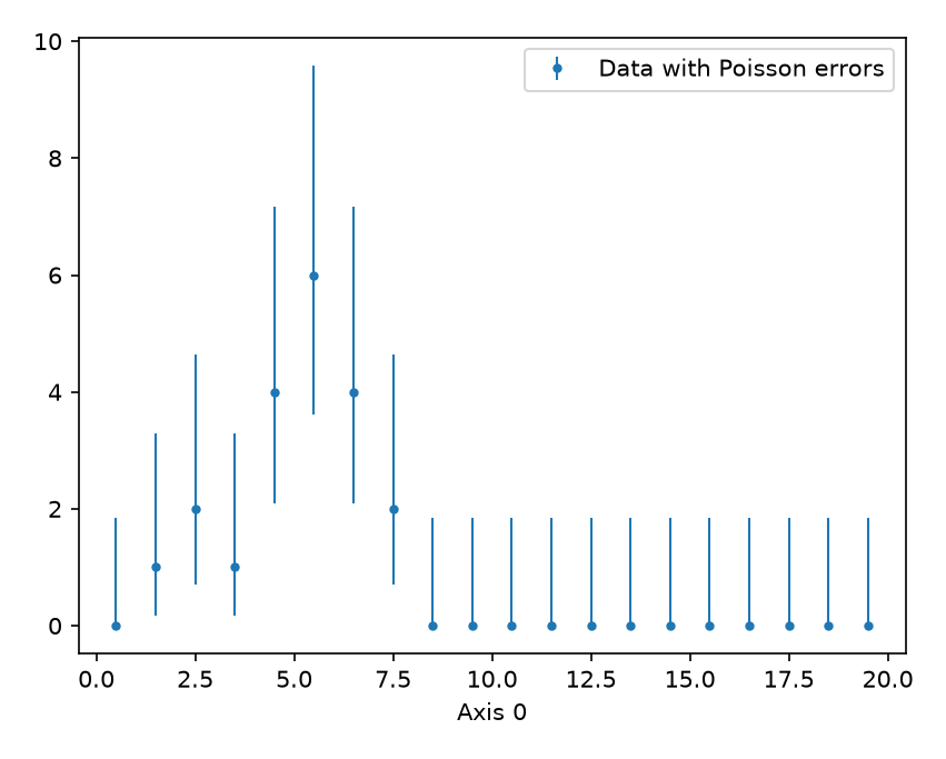
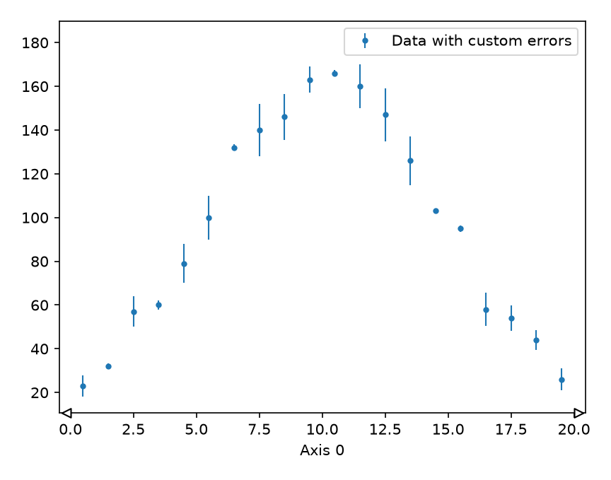
Control error bar display with yerr and w2method parameters:
# Simple histogram with Weight storage for automatic errors
h = hist.new.Reg(20, 0, 20).Weight().fill(np.random.poisson(5, 20))

fig, ax = plt.subplots()
mh.histplot(h, histtype='errorbar', yerr=True, label='Data with Poisson errors', ax=ax)
ax.legend(loc='upper right')
mh.yscale_legend(soft_fail=True)
# Simple histogram with custom error bars
h = hist.new.Reg(20, 0, 20).Weight().fill(np.random.normal(10, 5, 2000))
custom_errors = np.minimum(np.sqrt(h.values()), np.random.uniform(0, 20, 20))

fig, ax = plt.subplots()
mh.histplot(h, histtype='errorbar', yerr=custom_errors, label='Data with custom errors', ax=ax)
ax.legend(loc='upper right')
mh.yscale_legend(soft_fail=True)
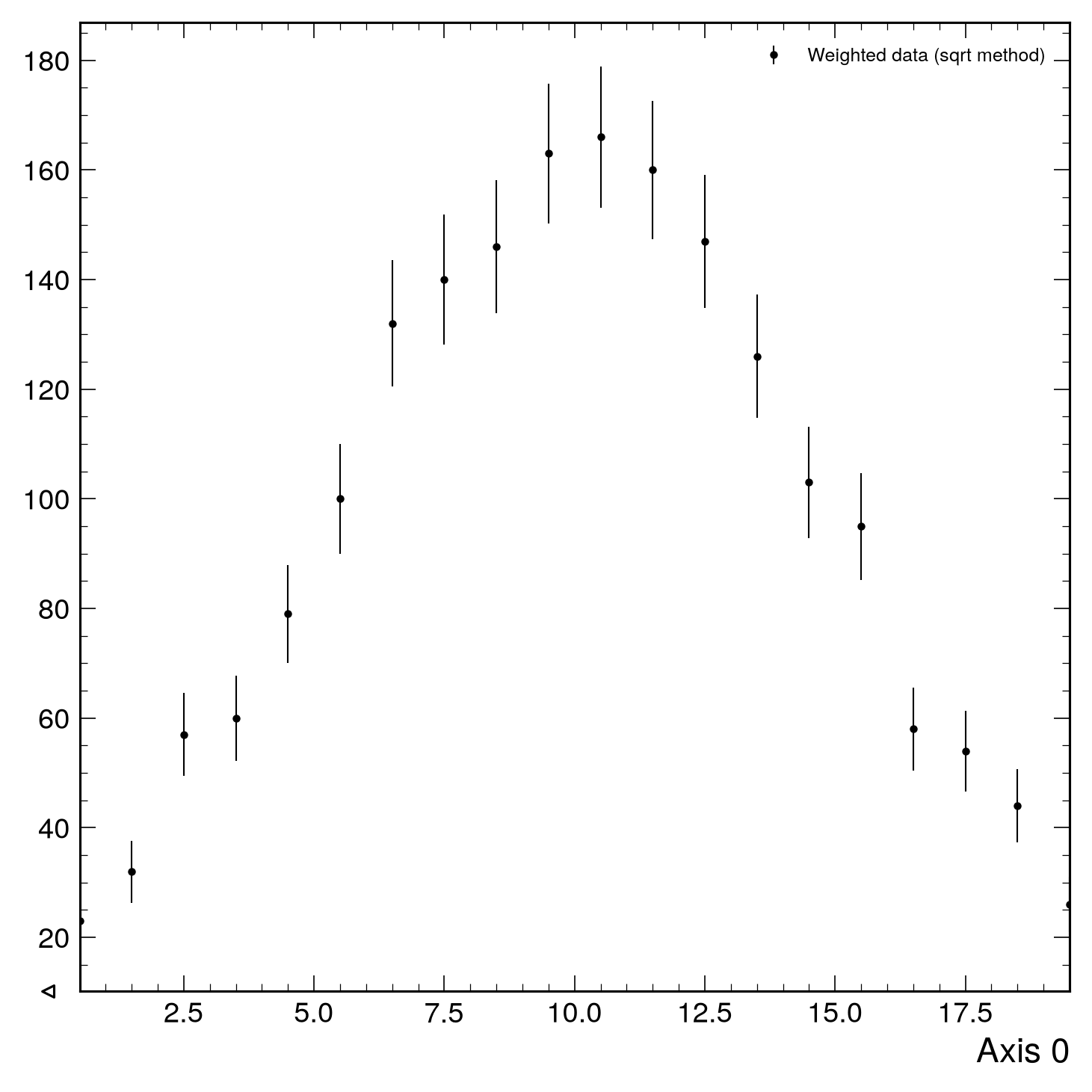
# Weighted histogram - errors from sqrt of sum of weights squared
h = hist.new.Reg(20, 0, 20).Weight().fill(np.random.normal(10, 5, 2000))

fig, ax = plt.subplots()
mh.histplot(h, histtype='errorbar', w2method='sqrt', label='Weighted data (sqrt method)', ax=ax)
ax.legend(loc='upper right')
mh.yscale_legend(soft_fail=True)
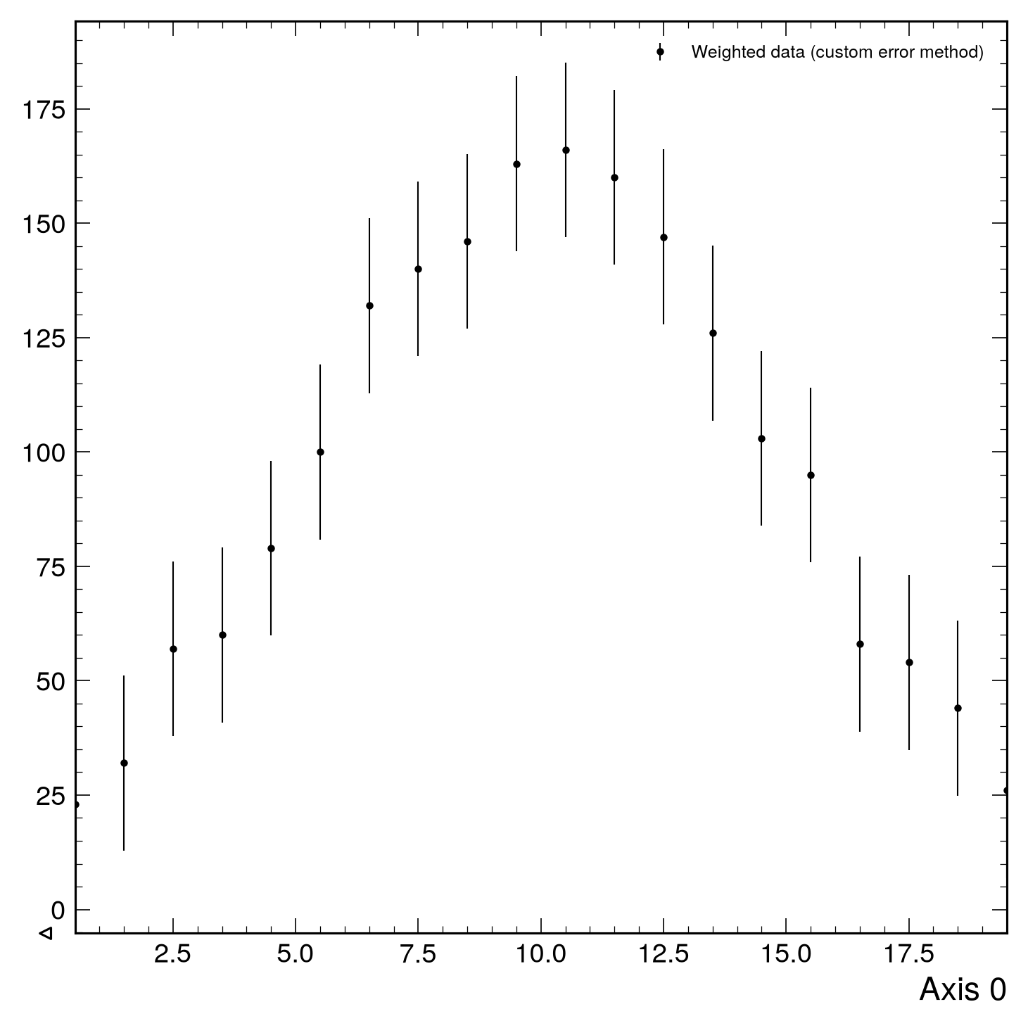
# Weighted histogram with custom error calculation
h = hist.new.Reg(20, 0, 20).Weight().fill(np.random.normal(10, 5, 2000))

# Custom error function: error = sqrt(sum(weights^2)) / 2
def custom_w2_method(weights, variances):
 up = weights - np.ones_like(weights) * 0.2 * np.mean(weights)
 down = weights + np.ones_like(weights) * 0.2 * np.mean(weights)
 return up, down

fig, ax = plt.subplots()
mh.histplot(h, histtype='errorbar', w2method=custom_w2_method, label='Weighted data (custom error method)', ax=ax)
ax.legend(loc='upper right')
mh.yscale_legend(soft_fail=True)
# Simple histogram with Weight storage for automatic errors
h = hist.new.Reg(20, 0, 20).Weight().fill(np.random.poisson(5, 20))

fig, ax = plt.subplots()
mh.histplot(h, histtype='errorbar', yerr=True, label='Data with Poisson errors', ax=ax)
ax.legend(loc='upper right')
mh.yscale_legend(soft_fail=True)
# Simple histogram with custom error bars
h = hist.new.Reg(20, 0, 20).Weight().fill(np.random.normal(10, 5, 2000))
custom_errors = np.minimum(np.sqrt(h.values()), np.random.uniform(0, 20, 20))

fig, ax = plt.subplots()
mh.histplot(h, histtype='errorbar', yerr=custom_errors, label='Data with custom errors', ax=ax)
ax.legend(loc='upper right')
mh.yscale_legend(soft_fail=True)
# Weighted histogram - errors from sqrt of sum of weights squared
h = hist.new.Reg(20, 0, 20).Weight().fill(np.random.normal(10, 5, 2000))

fig, ax = plt.subplots()
mh.histplot(h, histtype='errorbar', w2method='sqrt', label='Weighted data (sqrt method)', ax=ax)
ax.legend(loc='upper right')
mh.yscale_legend(soft_fail=True)
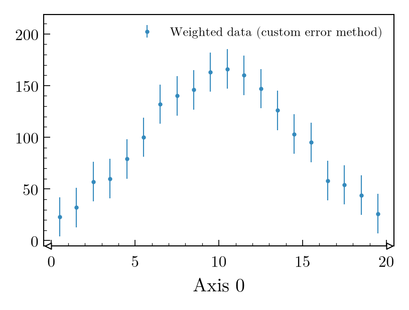
# Weighted histogram with custom error calculation
h = hist.new.Reg(20, 0, 20).Weight().fill(np.random.normal(10, 5, 2000))

# Custom error function: error = sqrt(sum(weights^2)) / 2
def custom_w2_method(weights, variances):
 up = weights - np.ones_like(weights) * 0.2 * np.mean(weights)
 down = weights + np.ones_like(weights) * 0.2 * np.mean(weights)
 return up, down

fig, ax = plt.subplots()
mh.histplot(h, histtype='errorbar', w2method=custom_w2_method, label='Weighted data (custom error method)', ax=ax)
ax.legend(loc='upper right')
mh.yscale_legend(soft_fail=True)
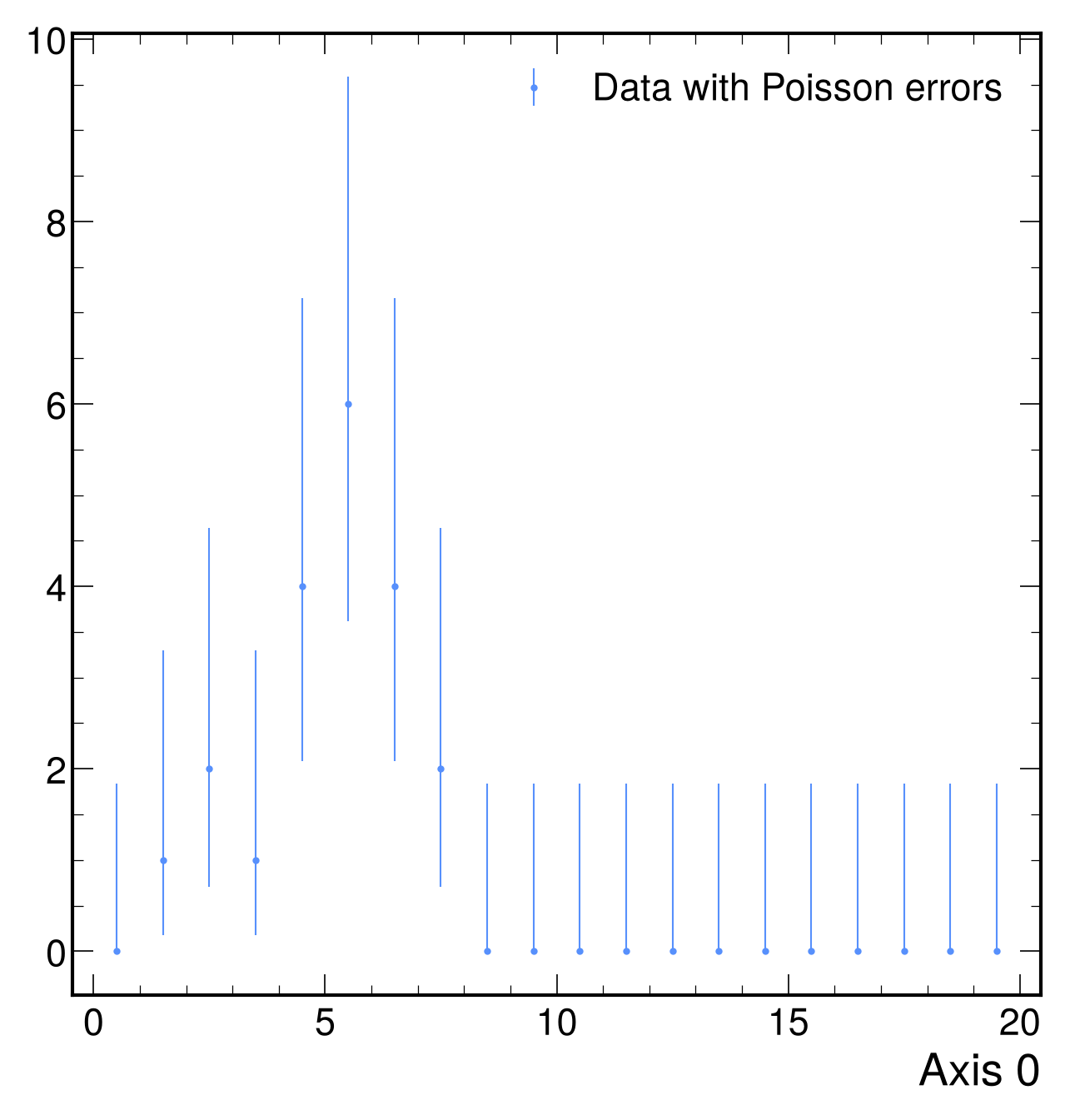
# Simple histogram with Weight storage for automatic errors
h = hist.new.Reg(20, 0, 20).Weight().fill(np.random.poisson(5, 20))

fig, ax = plt.subplots()
mh.histplot(h, histtype='errorbar', yerr=True, label='Data with Poisson errors', ax=ax)
ax.legend(loc='upper right')
mh.yscale_legend(soft_fail=True)
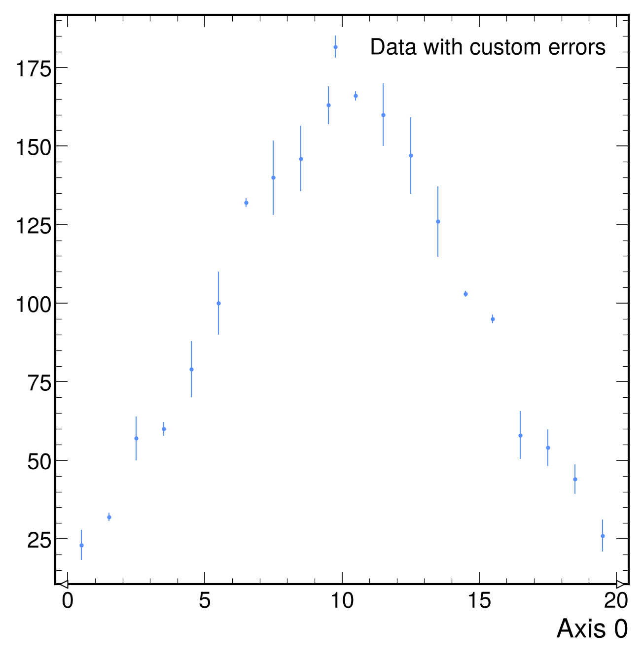
# Simple histogram with custom error bars
h = hist.new.Reg(20, 0, 20).Weight().fill(np.random.normal(10, 5, 2000))
custom_errors = np.minimum(np.sqrt(h.values()), np.random.uniform(0, 20, 20))

fig, ax = plt.subplots()
mh.histplot(h, histtype='errorbar', yerr=custom_errors, label='Data with custom errors', ax=ax)
ax.legend(loc='upper right')
mh.yscale_legend(soft_fail=True)
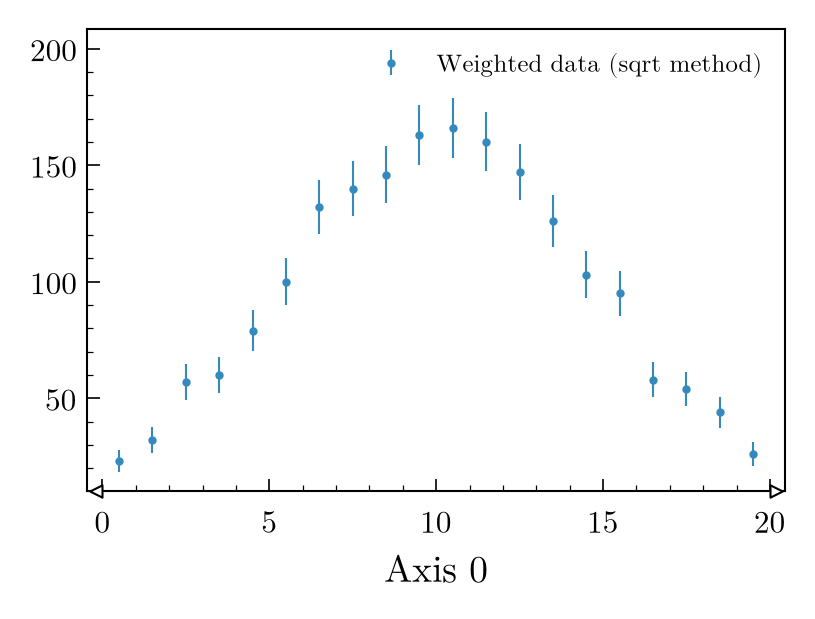
# Weighted histogram - errors from sqrt of sum of weights squared
h = hist.new.Reg(20, 0, 20).Weight().fill(np.random.normal(10, 5, 2000))
fig, ax = plt.subplots()
mh.histplot(h, histtype='errorbar', w2method='sqrt', label='Weighted data (sqrt method)', ax=ax)
ax.legend(loc='upper right')
mh.yscale_legend(soft_fail=True)
# Weighted histogram with custom error calculation
h = hist.new.Reg(20, 0, 20).Weight().fill(np.random.normal(10, 5, 2000))
# Custom error function: error = sqrt(sum(weights^2)) / 2
def custom_w2_method(weights, variances):
up = weights - np.ones_like(weights) * 0.2 * np.mean(weights)
down = weights + np.ones_like(weights) * 0.2 * np.mean(weights)
return up, down
fig, ax = plt.subplots()
mh.histplot(h, histtype='errorbar', w2method=custom_w2_method, label='Weighted data (custom error method)', ax=ax)
ax.legend(loc='upper right')
mh.yscale_legend(soft_fail=True)
# Simple histogram with Weight storage for automatic errors
h = hist.new.Reg(20, 0, 20).Weight().fill(np.random.poisson(5, 20))
fig, ax = plt.subplots()
mh.histplot(h, histtype='errorbar', yerr=True, label='Data with Poisson errors', ax=ax)
ax.legend(loc='upper right')
mh.yscale_legend(soft_fail=True)
# Simple histogram with custom error bars
h = hist.new.Reg(20, 0, 20).Weight().fill(np.random.normal(10, 5, 2000))
custom_errors = np.minimum(np.sqrt(h.values()), np.random.uniform(0, 20, 20))
fig, ax = plt.subplots()
mh.histplot(h, histtype='errorbar', yerr=custom_errors, label='Data with custom errors', ax=ax)
ax.legend(loc='upper right')
mh.yscale_legend(soft_fail=True)
# Weighted histogram - errors from sqrt of sum of weights squared
h = hist.new.Reg(20, 0, 20).Weight().fill(np.random.normal(10, 5, 2000))
fig, ax = plt.subplots()
mh.histplot(h, histtype='errorbar', w2method='sqrt', label='Weighted data (sqrt method)', ax=ax)
ax.legend(loc='upper right')
mh.yscale_legend(soft_fail=True)
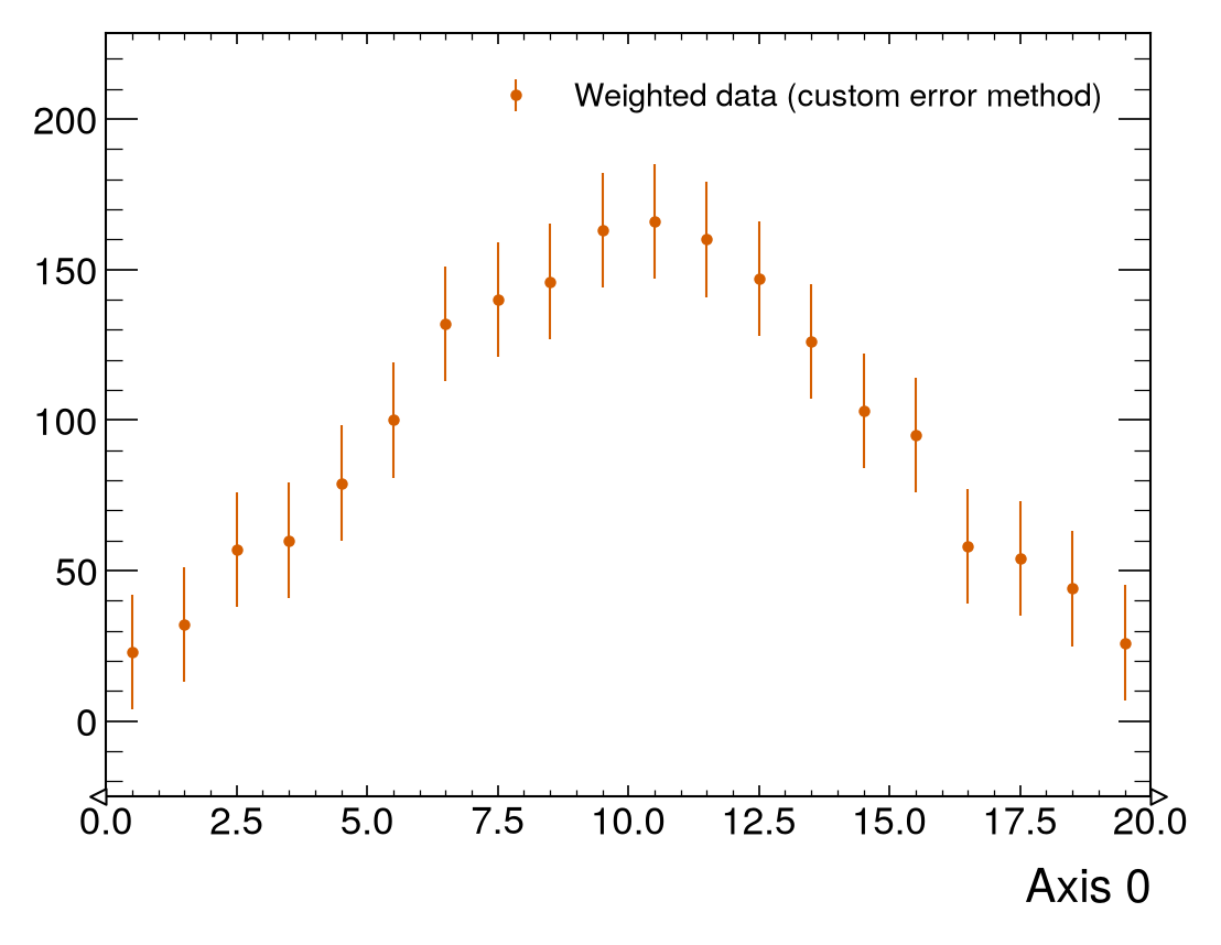
# Weighted histogram with custom error calculation
h = hist.new.Reg(20, 0, 20).Weight().fill(np.random.normal(10, 5, 2000))
# Custom error function: error = sqrt(sum(weights^2)) / 2
def custom_w2_method(weights, variances):
up = weights - np.ones_like(weights) * 0.2 * np.mean(weights)
down = weights + np.ones_like(weights) * 0.2 * np.mean(weights)
return up, down
fig, ax = plt.subplots()
mh.histplot(h, histtype='errorbar', w2method=custom_w2_method, label='Weighted data (custom error method)', ax=ax)
ax.legend(loc='upper right')
mh.yscale_legend(soft_fail=True)
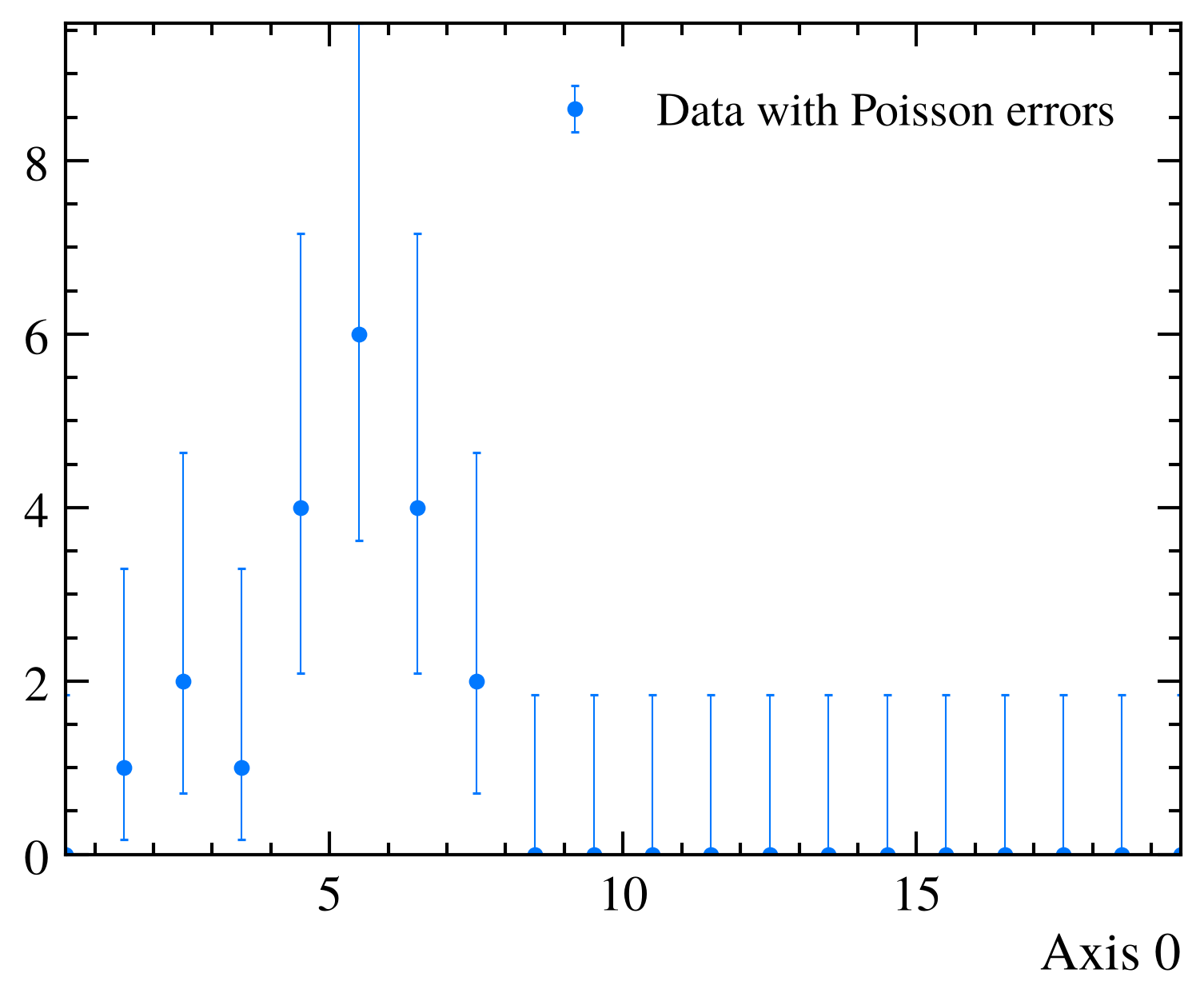
# Simple histogram with Weight storage for automatic errors
h = hist.new.Reg(20, 0, 20).Weight().fill(np.random.poisson(5, 20))
fig, ax = plt.subplots()
mh.histplot(h, histtype='errorbar', yerr=True, label='Data with Poisson errors', ax=ax)
ax.legend(loc='upper right')
mh.yscale_legend(soft_fail=True)
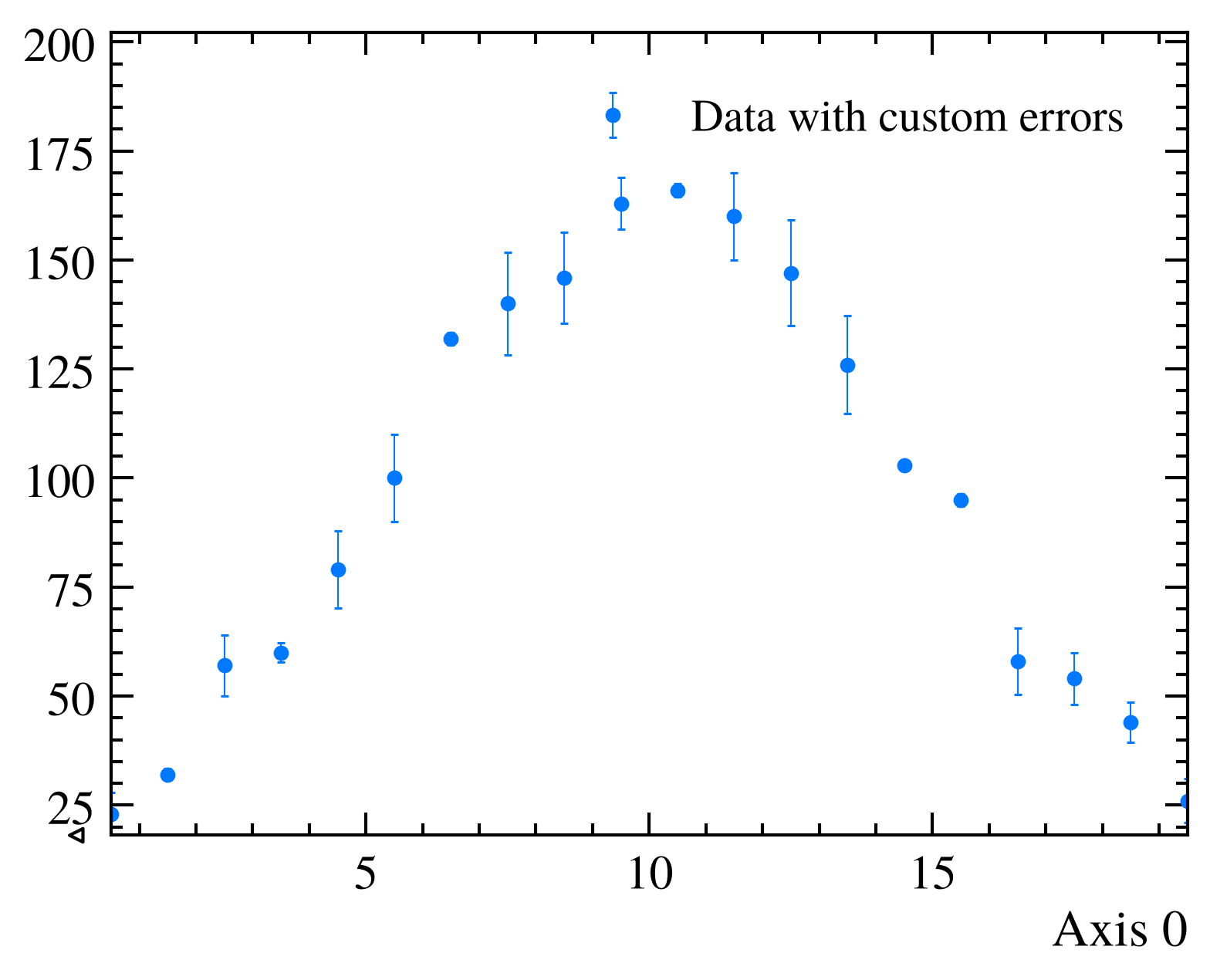
# Simple histogram with custom error bars
h = hist.new.Reg(20, 0, 20).Weight().fill(np.random.normal(10, 5, 2000))
custom_errors = np.minimum(np.sqrt(h.values()), np.random.uniform(0, 20, 20))
fig, ax = plt.subplots()
mh.histplot(h, histtype='errorbar', yerr=custom_errors, label='Data with custom errors', ax=ax)
ax.legend(loc='upper right')
mh.yscale_legend(soft_fail=True)
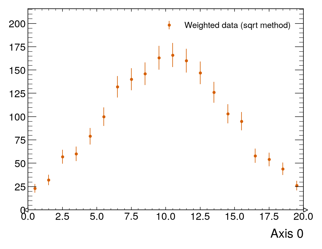
# Weighted histogram - errors from sqrt of sum of weights squared
h = hist.new.Reg(20, 0, 20).Weight().fill(np.random.normal(10, 5, 2000))
fig, ax = plt.subplots()
mh.histplot(h, histtype='errorbar', w2method='sqrt', label='Weighted data (sqrt method)', ax=ax)
ax.legend(loc='upper right')
mh.yscale_legend(soft_fail=True)
# Weighted histogram with custom error calculation
h = hist.new.Reg(20, 0, 20).Weight().fill(np.random.normal(10, 5, 2000))
# Custom error function: error = sqrt(sum(weights^2)) / 2
def custom_w2_method(weights, variances):
up = weights - np.ones_like(weights) * 0.2 * np.mean(weights)
down = weights + np.ones_like(weights) * 0.2 * np.mean(weights)
return up, down
fig, ax = plt.subplots()
mh.histplot(h, histtype='errorbar', w2method=custom_w2_method, label='Weighted data (custom error method)', ax=ax)
ax.legend(loc='upper right')
mh.yscale_legend(soft_fail=True)
# Simple histogram with Weight storage for automatic errors
h = hist.new.Reg(20, 0, 20).Weight().fill(np.random.poisson(5, 20))
fig, ax = plt.subplots()
mh.histplot(h, histtype='errorbar', yerr=True, label='Data with Poisson errors', ax=ax)
ax.legend(loc='upper right')
mh.yscale_legend(soft_fail=True)
# Simple histogram with custom error bars
h = hist.new.Reg(20, 0, 20).Weight().fill(np.random.normal(10, 5, 2000))
custom_errors = np.minimum(np.sqrt(h.values()), np.random.uniform(0, 20, 20))
fig, ax = plt.subplots()
mh.histplot(h, histtype='errorbar', yerr=custom_errors, label='Data with custom errors', ax=ax)
ax.legend(loc='upper right')
mh.yscale_legend(soft_fail=True)
# Weighted histogram - errors from sqrt of sum of weights squared
h = hist.new.Reg(20, 0, 20).Weight().fill(np.random.normal(10, 5, 2000))
fig, ax = plt.subplots()
mh.histplot(h, histtype='errorbar', w2method='sqrt', label='Weighted data (sqrt method)', ax=ax)
ax.legend(loc='upper right')
mh.yscale_legend(soft_fail=True)
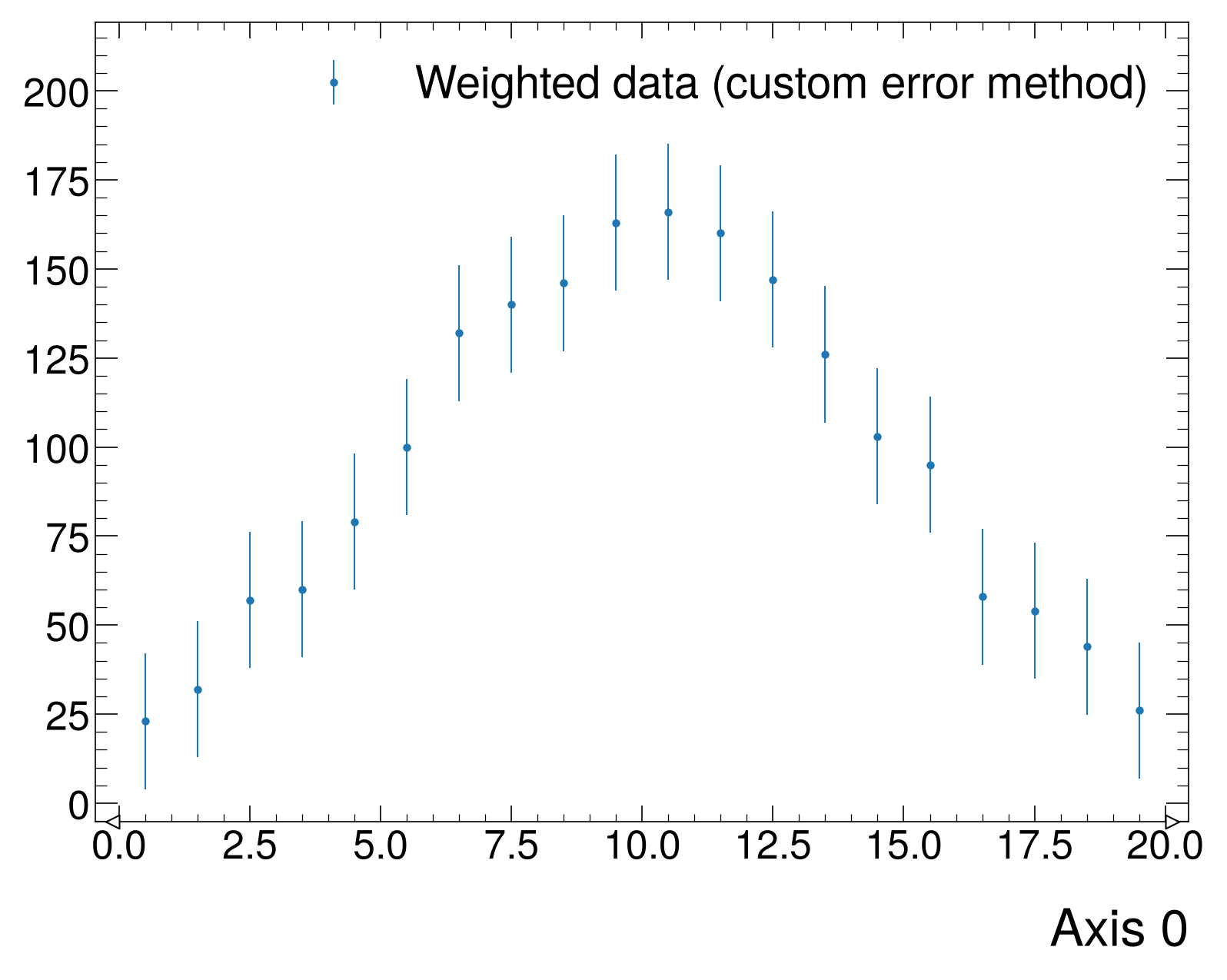
# Weighted histogram with custom error calculation
h = hist.new.Reg(20, 0, 20).Weight().fill(np.random.normal(10, 5, 2000))
# Custom error function: error = sqrt(sum(weights^2)) / 2
def custom_w2_method(weights, variances):
up = weights - np.ones_like(weights) * 0.2 * np.mean(weights)
down = weights + np.ones_like(weights) * 0.2 * np.mean(weights)
return up, down
fig, ax = plt.subplots()
mh.histplot(h, histtype='errorbar', w2method=custom_w2_method, label='Weighted data (custom error method)', ax=ax)
ax.legend(loc='upper right')
mh.yscale_legend(soft_fail=True)
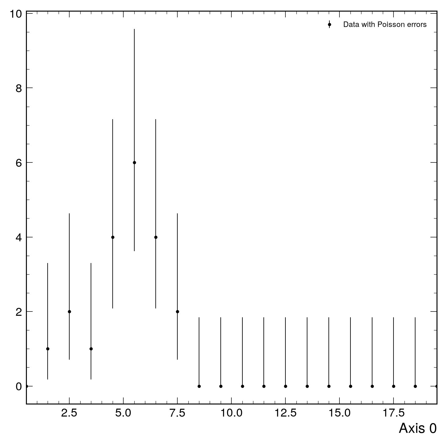
# Simple histogram with Weight storage for automatic errors
h = hist.new.Reg(20, 0, 20).Weight().fill(np.random.poisson(5, 20))
fig, ax = plt.subplots()
mh.histplot(h, histtype='errorbar', yerr=True, label='Data with Poisson errors', ax=ax)
ax.legend(loc='upper right')
mh.yscale_legend(soft_fail=True)
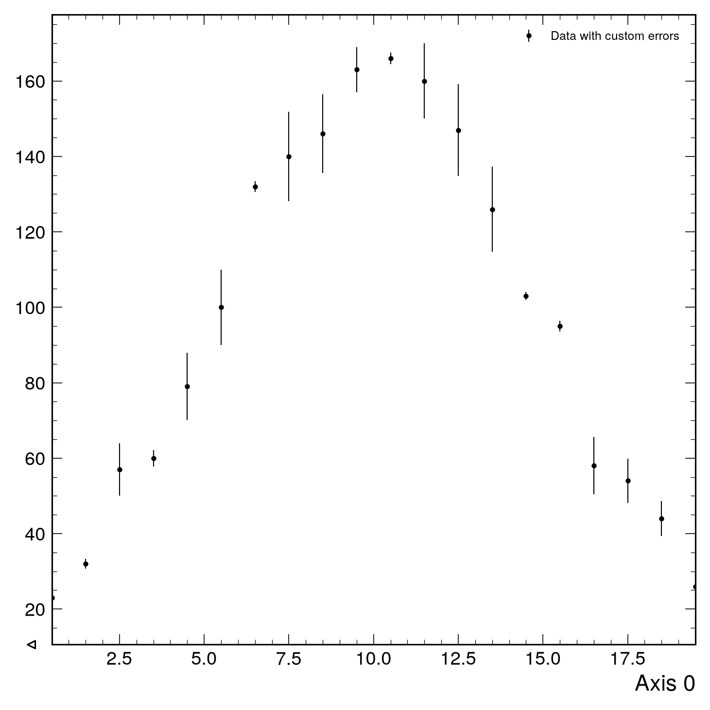
# Simple histogram with custom error bars
h = hist.new.Reg(20, 0, 20).Weight().fill(np.random.normal(10, 5, 2000))
custom_errors = np.minimum(np.sqrt(h.values()), np.random.uniform(0, 20, 20))
fig, ax = plt.subplots()
mh.histplot(h, histtype='errorbar', yerr=custom_errors, label='Data with custom errors', ax=ax)
ax.legend(loc='upper right')
mh.yscale_legend(soft_fail=True)
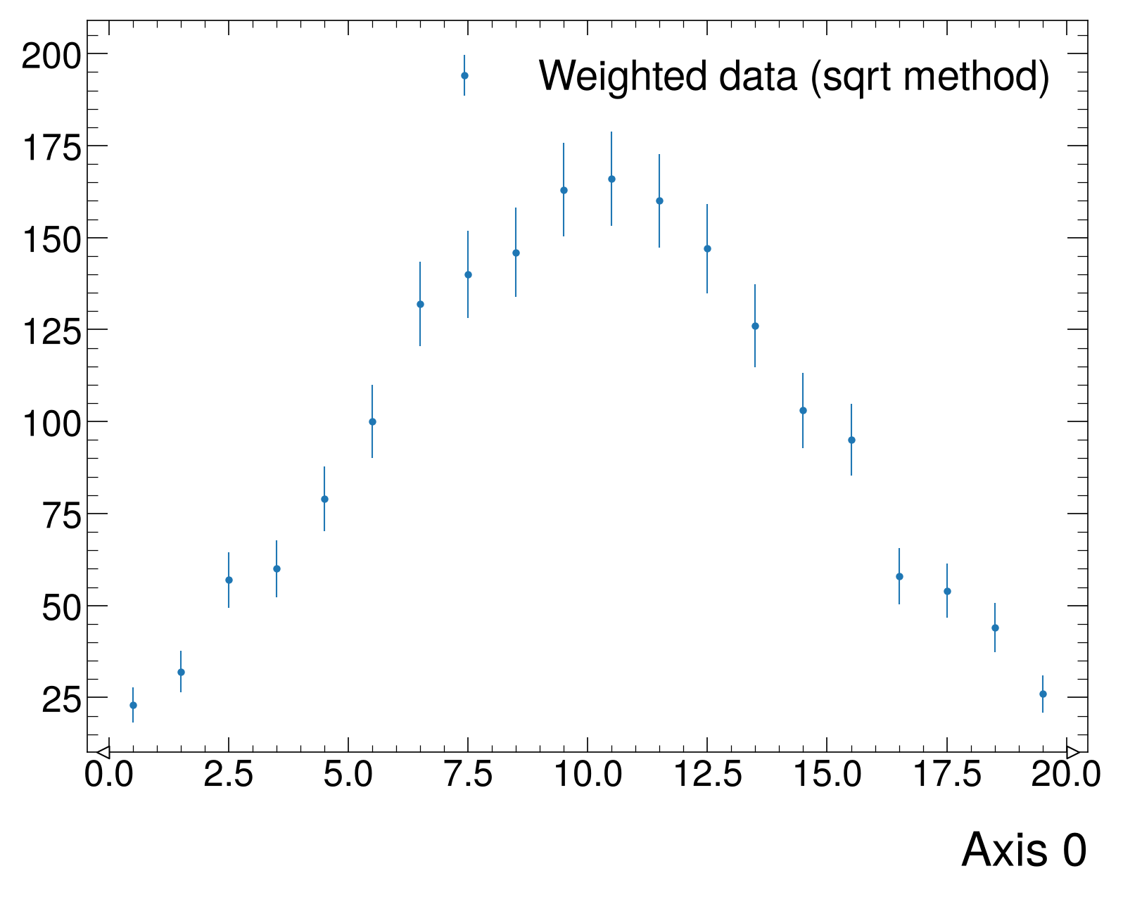
# Weighted histogram - errors from sqrt of sum of weights squared
h = hist.new.Reg(20, 0, 20).Weight().fill(np.random.normal(10, 5, 2000))
fig, ax = plt.subplots()
mh.histplot(h, histtype='errorbar', w2method='sqrt', label='Weighted data (sqrt method)', ax=ax)
ax.legend(loc='upper right')
mh.yscale_legend(soft_fail=True)
# Weighted histogram with custom error calculation
h = hist.new.Reg(20, 0, 20).Weight().fill(np.random.normal(10, 5, 2000))
# Custom error function: error = sqrt(sum(weights^2)) / 2
def custom_w2_method(weights, variances):
up = weights - np.ones_like(weights) * 0.2 * np.mean(weights)
down = weights + np.ones_like(weights) * 0.2 * np.mean(weights)
return up, down
fig, ax = plt.subplots()
mh.histplot(h, histtype='errorbar', w2method=custom_w2_method, label='Weighted data (custom error method)', ax=ax)
ax.legend(loc='upper right')
mh.yscale_legend(soft_fail=True)
Normalization Options¤
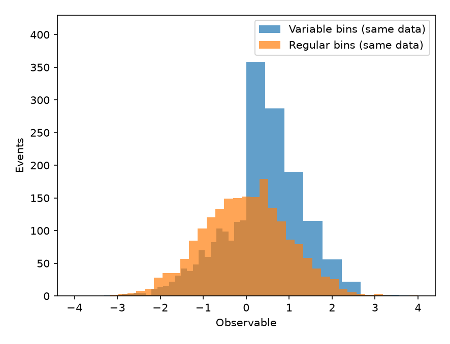
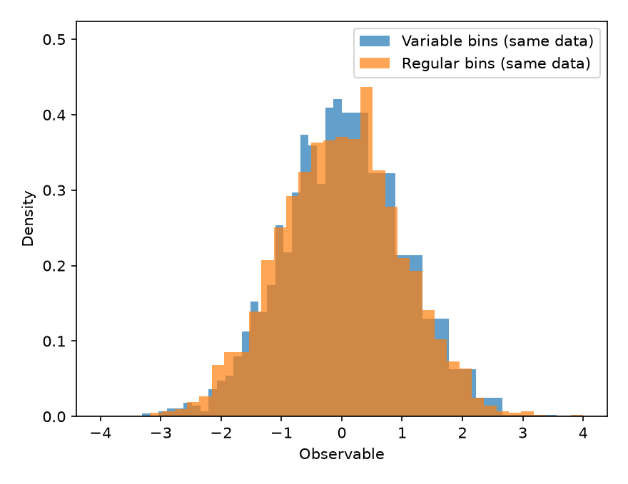
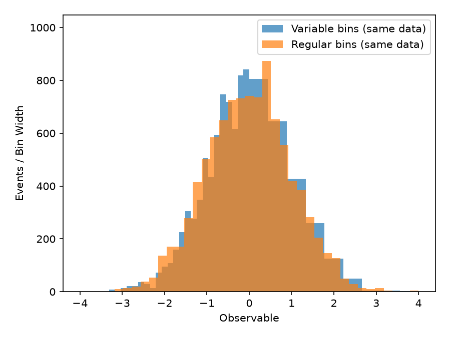
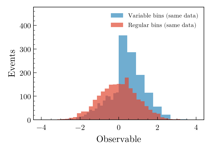
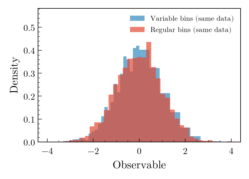
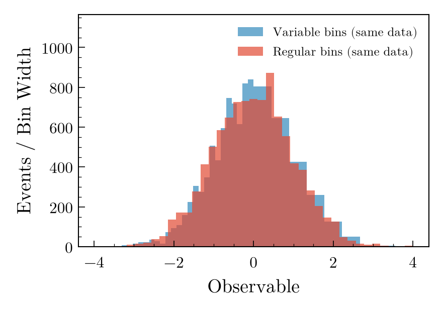
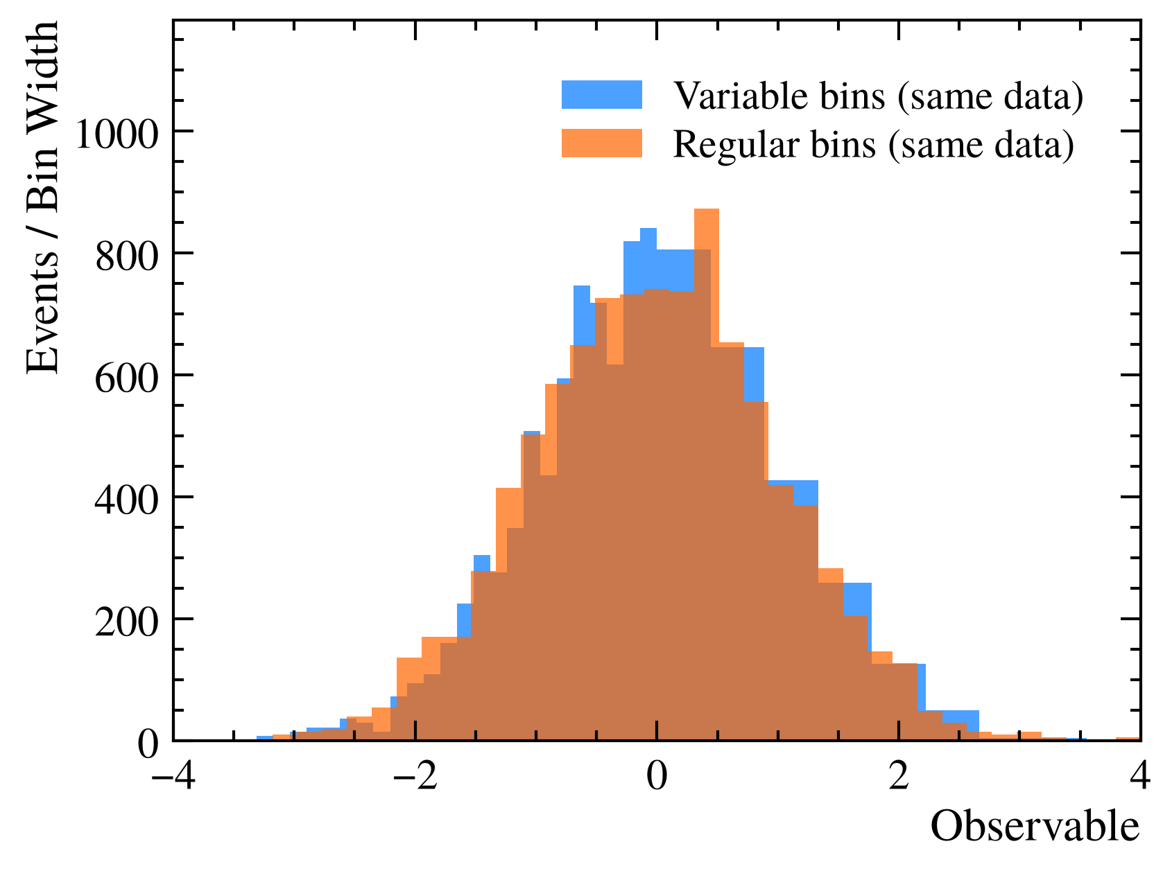
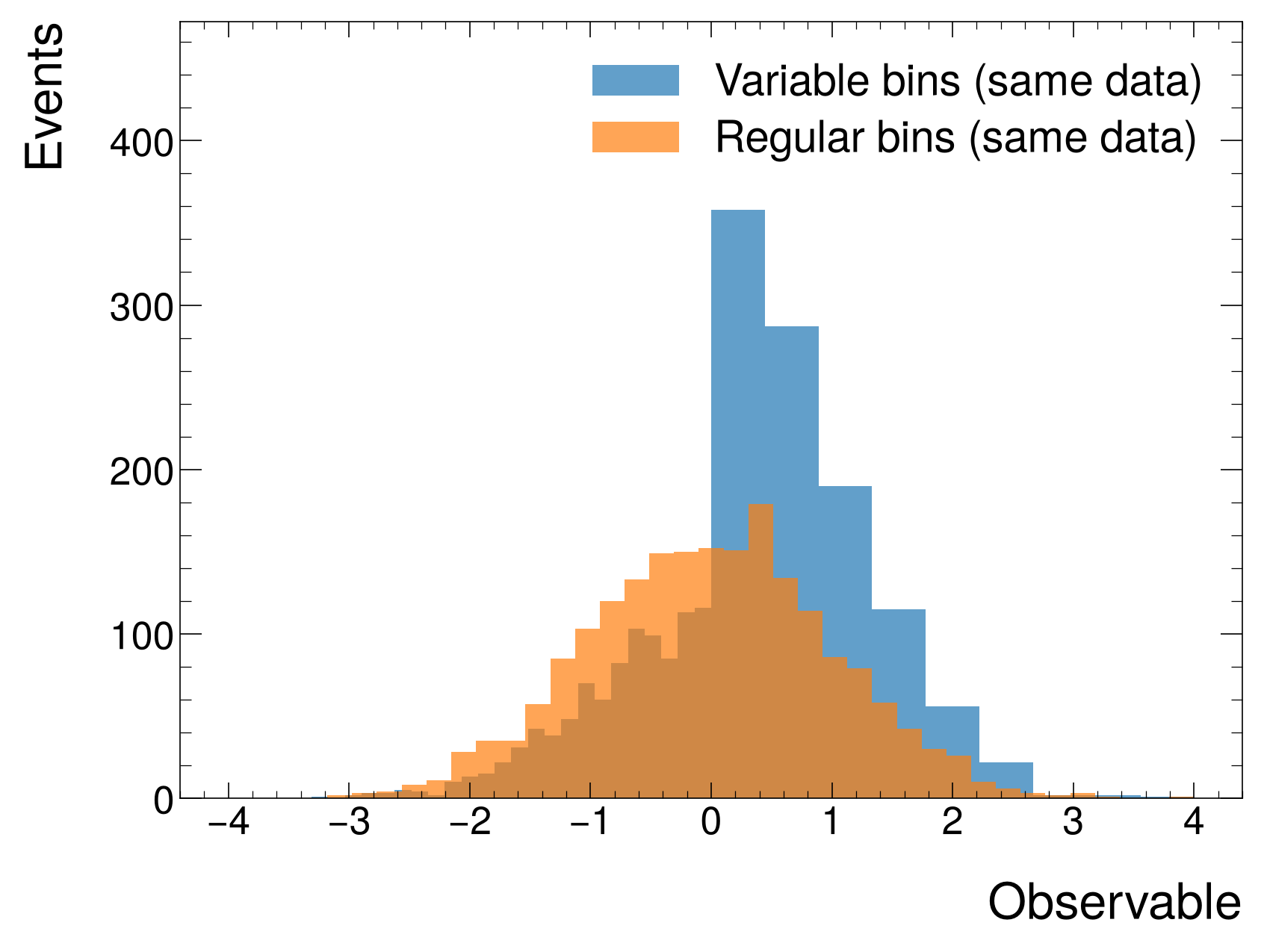
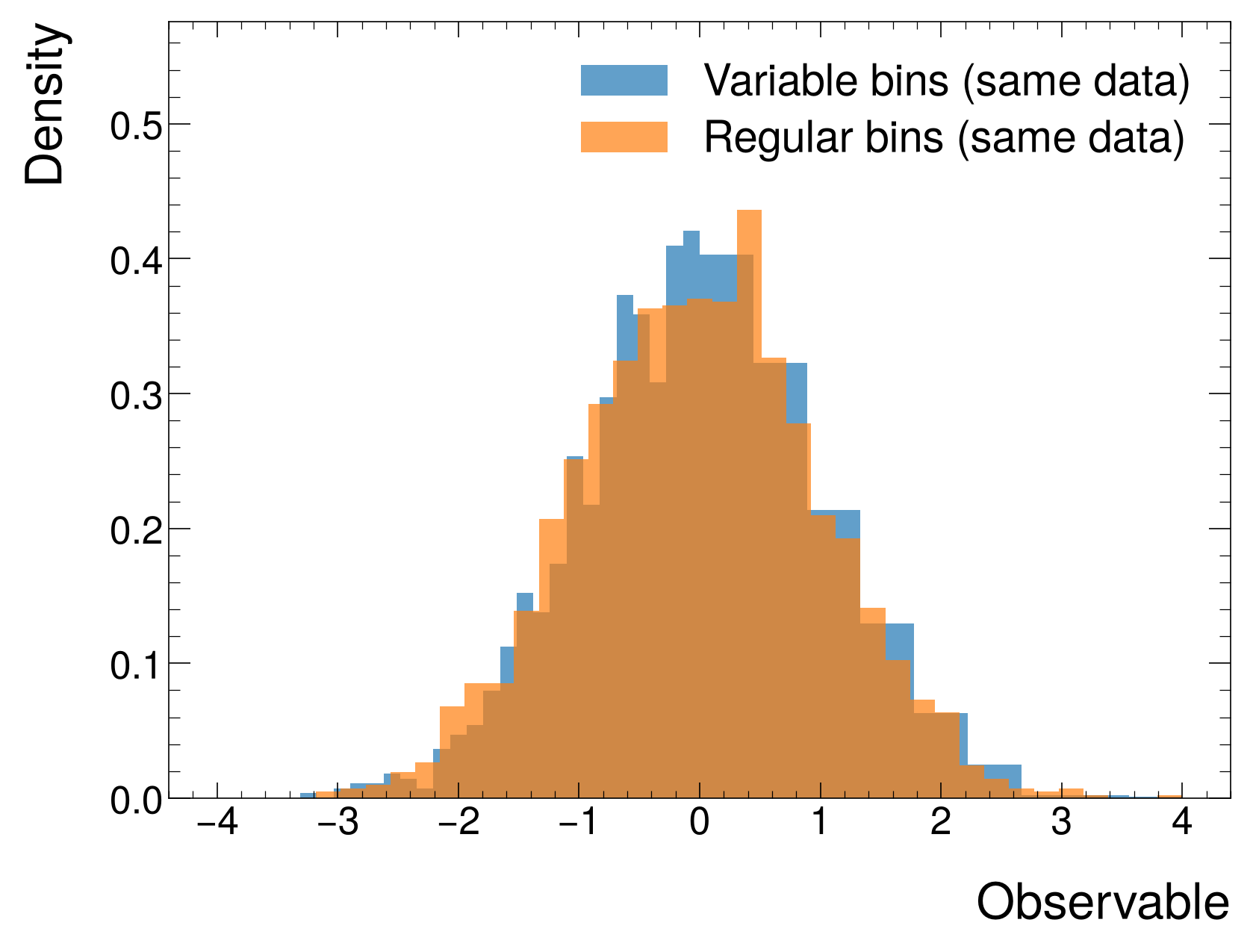
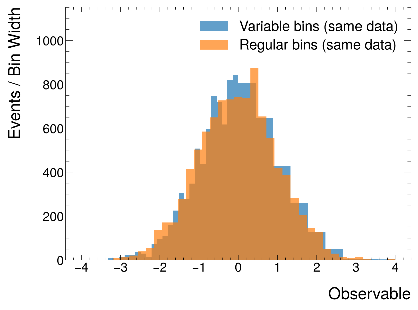
Control histogram normalization with density and binwnorm parameters:
# Create histograms with different binning schemes
bins1 = np.r_[np.linspace(-4, 0, 30)[:-1], np.linspace(0, 4, 10)] # Variable binning
bins2 = np.linspace(-4, 4, 40) # Regular binning
h1 = hist.new.Var(bins1).Weight().fill(np.random.normal(0, 1, 2000))
h2 = hist.new.Var(bins2).Weight().fill(np.random.normal(0, 1, 2000))
# Plot
kwargs = {}
fig, ax = plt.subplots()
mh.histplot(h1, histtype='fill', alpha=0.7, label='Variable bins (same data)', ax=ax, **kwargs)
mh.histplot(h2, histtype='fill', alpha=0.7, label='Regular bins (same data)', ax=ax, **kwargs)
# Style
ax.set_xlabel('Observable')
ax.set_ylabel('Events')
ax.legend(loc='upper right')
mh.yscale_legend(soft_fail=True)
# Create histograms with different binning schemes
bins1 = np.r_[np.linspace(-4, 0, 30)[:-1], np.linspace(0, 4, 10)] # Variable binning
bins2 = np.linspace(-4, 4, 40) # Regular binning
h1 = hist.new.Var(bins1).Weight().fill(np.random.normal(0, 1, 2000))
h2 = hist.new.Var(bins2).Weight().fill(np.random.normal(0, 1, 2000))
# Plot
kwargs = {'density': True}
fig, ax = plt.subplots()
mh.histplot(h1, histtype='fill', alpha=0.7, label='Variable bins (same data)', ax=ax, **kwargs)
mh.histplot(h2, histtype='fill', alpha=0.7, label='Regular bins (same data)', ax=ax, **kwargs)
# Style
ax.set_xlabel('Observable')
ax.set_ylabel('Density')
ax.legend(loc='upper right')
mh.yscale_legend(soft_fail=True)
# Create histograms with different binning schemes
bins1 = np.r_[np.linspace(-4, 0, 30)[:-1], np.linspace(0, 4, 10)] # Variable binning
bins2 = np.linspace(-4, 4, 40) # Regular binning
h1 = hist.new.Var(bins1).Weight().fill(np.random.normal(0, 1, 2000))
h2 = hist.new.Var(bins2).Weight().fill(np.random.normal(0, 1, 2000))
# Plot
kwargs = {'binwnorm': True}
fig, ax = plt.subplots()
mh.histplot(h1, histtype='fill', alpha=0.7, label='Variable bins (same data)', ax=ax, **kwargs)
mh.histplot(h2, histtype='fill', alpha=0.7, label='Regular bins (same data)', ax=ax, **kwargs)
# Style
ax.set_xlabel('Observable')
ax.set_ylabel('Events / Bin Width')
ax.legend(loc='upper right')
mh.yscale_legend(soft_fail=True)
# Create histograms with different binning schemes
bins1 = np.r_[np.linspace(-4, 0, 30)[:-1], np.linspace(0, 4, 10)] # Variable binning
bins2 = np.linspace(-4, 4, 40) # Regular binning
h1 = hist.new.Var(bins1).Weight().fill(np.random.normal(0, 1, 2000))
h2 = hist.new.Var(bins2).Weight().fill(np.random.normal(0, 1, 2000))
# Plot
kwargs = {}
fig, ax = plt.subplots()
mh.histplot(h1, histtype='fill', alpha=0.7, label='Variable bins (same data)', ax=ax, **kwargs)
mh.histplot(h2, histtype='fill', alpha=0.7, label='Regular bins (same data)', ax=ax, **kwargs)
# Style
ax.set_xlabel('Observable')
ax.set_ylabel('Events')
ax.legend(loc='upper right')
mh.yscale_legend(soft_fail=True)
# Create histograms with different binning schemes
bins1 = np.r_[np.linspace(-4, 0, 30)[:-1], np.linspace(0, 4, 10)] # Variable binning
bins2 = np.linspace(-4, 4, 40) # Regular binning
h1 = hist.new.Var(bins1).Weight().fill(np.random.normal(0, 1, 2000))
h2 = hist.new.Var(bins2).Weight().fill(np.random.normal(0, 1, 2000))
# Plot
kwargs = {'density': True}
fig, ax = plt.subplots()
mh.histplot(h1, histtype='fill', alpha=0.7, label='Variable bins (same data)', ax=ax, **kwargs)
mh.histplot(h2, histtype='fill', alpha=0.7, label='Regular bins (same data)', ax=ax, **kwargs)
# Style
ax.set_xlabel('Observable')
ax.set_ylabel('Density')
ax.legend(loc='upper right')
mh.yscale_legend(soft_fail=True)
# Create histograms with different binning schemes
bins1 = np.r_[np.linspace(-4, 0, 30)[:-1], np.linspace(0, 4, 10)] # Variable binning
bins2 = np.linspace(-4, 4, 40) # Regular binning
h1 = hist.new.Var(bins1).Weight().fill(np.random.normal(0, 1, 2000))
h2 = hist.new.Var(bins2).Weight().fill(np.random.normal(0, 1, 2000))
# Plot
kwargs = {'binwnorm': True}
fig, ax = plt.subplots()
mh.histplot(h1, histtype='fill', alpha=0.7, label='Variable bins (same data)', ax=ax, **kwargs)
mh.histplot(h2, histtype='fill', alpha=0.7, label='Regular bins (same data)', ax=ax, **kwargs)
# Style
ax.set_xlabel('Observable')
ax.set_ylabel('Events / Bin Width')
ax.legend(loc='upper right')
mh.yscale_legend(soft_fail=True)
# Create histograms with different binning schemes
bins1 = np.r_[np.linspace(-4, 0, 30)[:-1], np.linspace(0, 4, 10)] # Variable binning
bins2 = np.linspace(-4, 4, 40) # Regular binning
h1 = hist.new.Var(bins1).Weight().fill(np.random.normal(0, 1, 2000))
h2 = hist.new.Var(bins2).Weight().fill(np.random.normal(0, 1, 2000))
# Plot
kwargs = {}
fig, ax = plt.subplots()
mh.histplot(h1, histtype='fill', alpha=0.7, label='Variable bins (same data)', ax=ax, **kwargs)
mh.histplot(h2, histtype='fill', alpha=0.7, label='Regular bins (same data)', ax=ax, **kwargs)
# Style
ax.set_xlabel('Observable')
ax.set_ylabel('Events')
ax.legend(loc='upper right')
mh.yscale_legend(soft_fail=True)
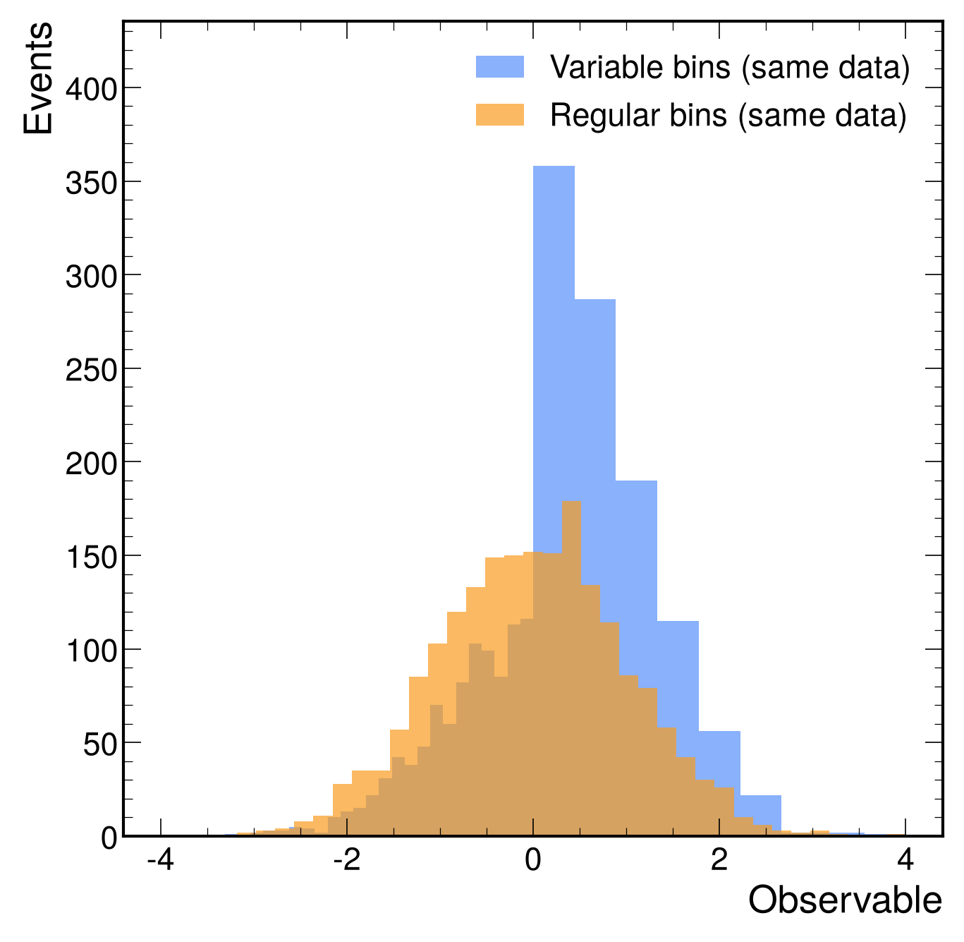
# Create histograms with different binning schemes
bins1 = np.r_[np.linspace(-4, 0, 30)[:-1], np.linspace(0, 4, 10)] # Variable binning
bins2 = np.linspace(-4, 4, 40) # Regular binning
h1 = hist.new.Var(bins1).Weight().fill(np.random.normal(0, 1, 2000))
h2 = hist.new.Var(bins2).Weight().fill(np.random.normal(0, 1, 2000))
# Plot
kwargs = {'density': True}
fig, ax = plt.subplots()
mh.histplot(h1, histtype='fill', alpha=0.7, label='Variable bins (same data)', ax=ax, **kwargs)
mh.histplot(h2, histtype='fill', alpha=0.7, label='Regular bins (same data)', ax=ax, **kwargs)
# Style
ax.set_xlabel('Observable')
ax.set_ylabel('Density')
ax.legend(loc='upper right')
mh.yscale_legend(soft_fail=True)
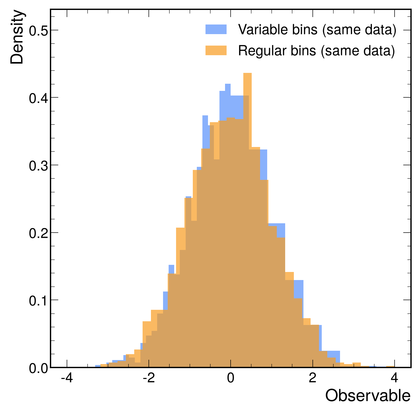
# Create histograms with different binning schemes
bins1 = np.r_[np.linspace(-4, 0, 30)[:-1], np.linspace(0, 4, 10)] # Variable binning
bins2 = np.linspace(-4, 4, 40) # Regular binning
h1 = hist.new.Var(bins1).Weight().fill(np.random.normal(0, 1, 2000))
h2 = hist.new.Var(bins2).Weight().fill(np.random.normal(0, 1, 2000))
# Plot
kwargs = {'binwnorm': True}
fig, ax = plt.subplots()
mh.histplot(h1, histtype='fill', alpha=0.7, label='Variable bins (same data)', ax=ax, **kwargs)
mh.histplot(h2, histtype='fill', alpha=0.7, label='Regular bins (same data)', ax=ax, **kwargs)
# Style
ax.set_xlabel('Observable')
ax.set_ylabel('Events / Bin Width')
ax.legend(loc='upper right')
mh.yscale_legend(soft_fail=True)
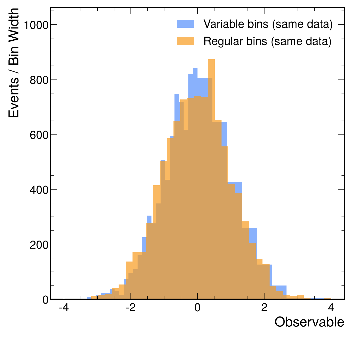
# Create histograms with different binning schemes
bins1 = np.r_[np.linspace(-4, 0, 30)[:-1], np.linspace(0, 4, 10)] # Variable binning
bins2 = np.linspace(-4, 4, 40) # Regular binning
h1 = hist.new.Var(bins1).Weight().fill(np.random.normal(0, 1, 2000))
h2 = hist.new.Var(bins2).Weight().fill(np.random.normal(0, 1, 2000))
# Plot
kwargs = {}
fig, ax = plt.subplots()
mh.histplot(h1, histtype='fill', alpha=0.7, label='Variable bins (same data)', ax=ax, **kwargs)
mh.histplot(h2, histtype='fill', alpha=0.7, label='Regular bins (same data)', ax=ax, **kwargs)
# Style
ax.set_xlabel('Observable')
ax.set_ylabel('Events')
ax.legend(loc='upper right')
mh.yscale_legend(soft_fail=True)
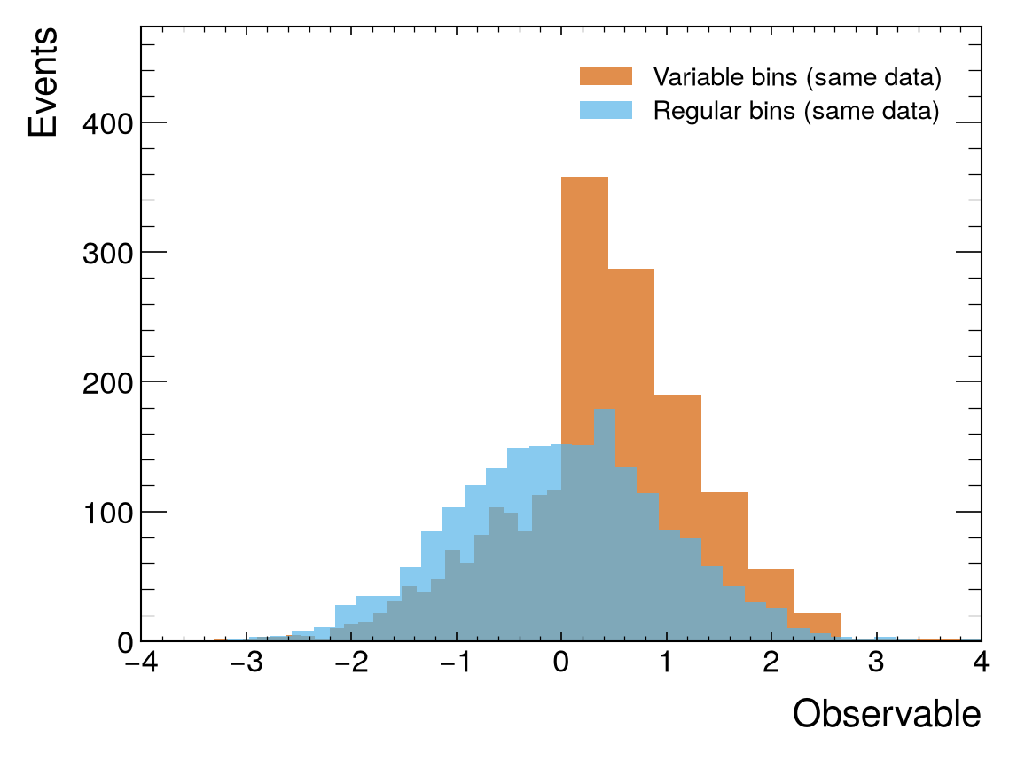
# Create histograms with different binning schemes
bins1 = np.r_[np.linspace(-4, 0, 30)[:-1], np.linspace(0, 4, 10)] # Variable binning
bins2 = np.linspace(-4, 4, 40) # Regular binning
h1 = hist.new.Var(bins1).Weight().fill(np.random.normal(0, 1, 2000))
h2 = hist.new.Var(bins2).Weight().fill(np.random.normal(0, 1, 2000))
# Plot
kwargs = {'density': True}
fig, ax = plt.subplots()
mh.histplot(h1, histtype='fill', alpha=0.7, label='Variable bins (same data)', ax=ax, **kwargs)
mh.histplot(h2, histtype='fill', alpha=0.7, label='Regular bins (same data)', ax=ax, **kwargs)
# Style
ax.set_xlabel('Observable')
ax.set_ylabel('Density')
ax.legend(loc='upper right')
mh.yscale_legend(soft_fail=True)
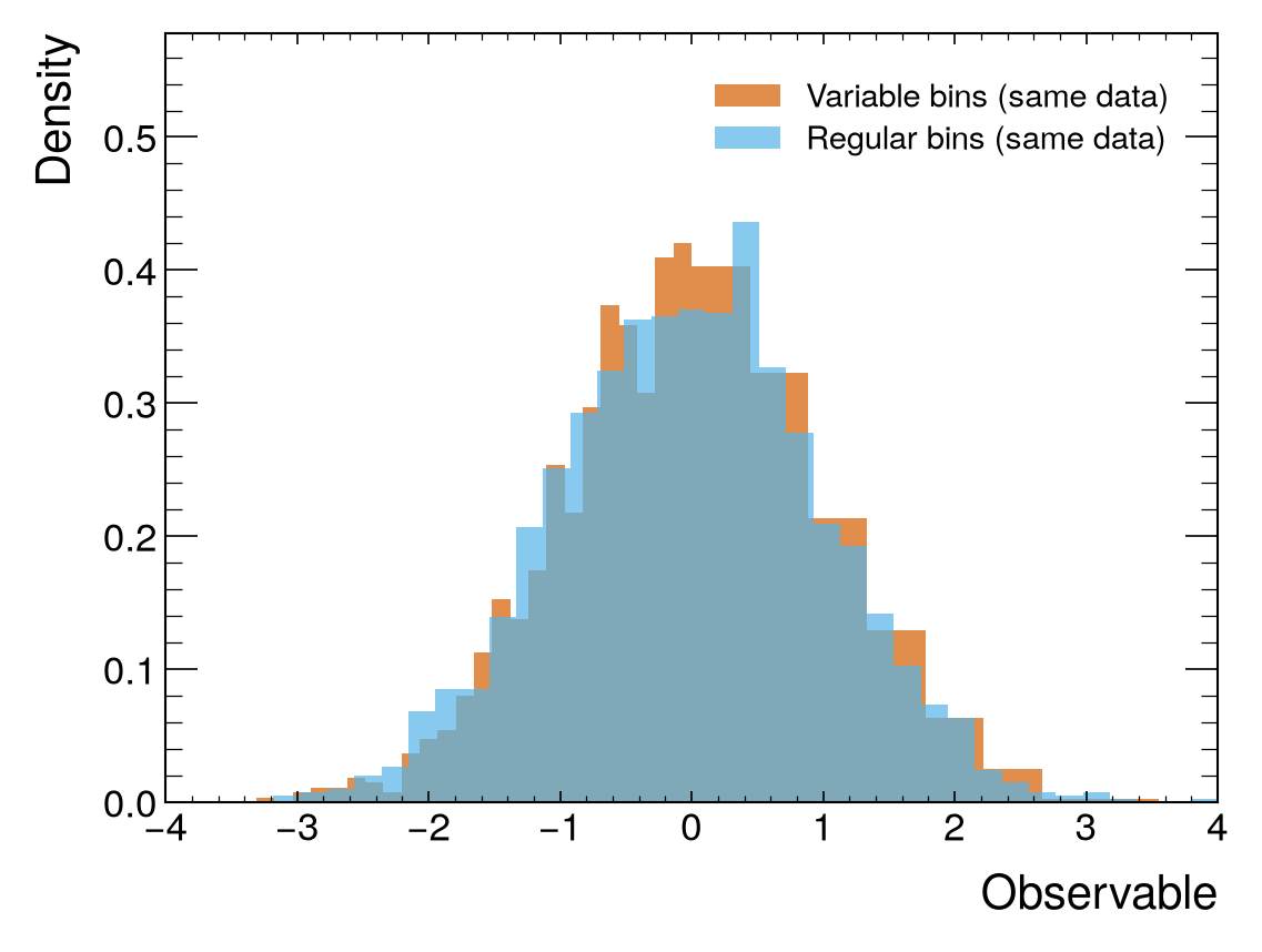
# Create histograms with different binning schemes
bins1 = np.r_[np.linspace(-4, 0, 30)[:-1], np.linspace(0, 4, 10)] # Variable binning
bins2 = np.linspace(-4, 4, 40) # Regular binning
h1 = hist.new.Var(bins1).Weight().fill(np.random.normal(0, 1, 2000))
h2 = hist.new.Var(bins2).Weight().fill(np.random.normal(0, 1, 2000))
# Plot
kwargs = {'binwnorm': True}
fig, ax = plt.subplots()
mh.histplot(h1, histtype='fill', alpha=0.7, label='Variable bins (same data)', ax=ax, **kwargs)
mh.histplot(h2, histtype='fill', alpha=0.7, label='Regular bins (same data)', ax=ax, **kwargs)
# Style
ax.set_xlabel('Observable')
ax.set_ylabel('Events / Bin Width')
ax.legend(loc='upper right')
mh.yscale_legend(soft_fail=True)
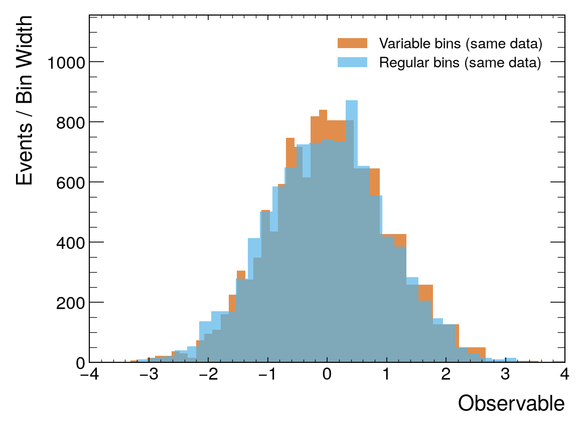
# Create histograms with different binning schemes
bins1 = np.r_[np.linspace(-4, 0, 30)[:-1], np.linspace(0, 4, 10)] # Variable binning
bins2 = np.linspace(-4, 4, 40) # Regular binning
h1 = hist.new.Var(bins1).Weight().fill(np.random.normal(0, 1, 2000))
h2 = hist.new.Var(bins2).Weight().fill(np.random.normal(0, 1, 2000))
# Plot
kwargs = {}
fig, ax = plt.subplots()
mh.histplot(h1, histtype='fill', alpha=0.7, label='Variable bins (same data)', ax=ax, **kwargs)
mh.histplot(h2, histtype='fill', alpha=0.7, label='Regular bins (same data)', ax=ax, **kwargs)
# Style
ax.set_xlabel('Observable')
ax.set_ylabel('Events')
ax.legend(loc='upper right')
mh.yscale_legend(soft_fail=True)
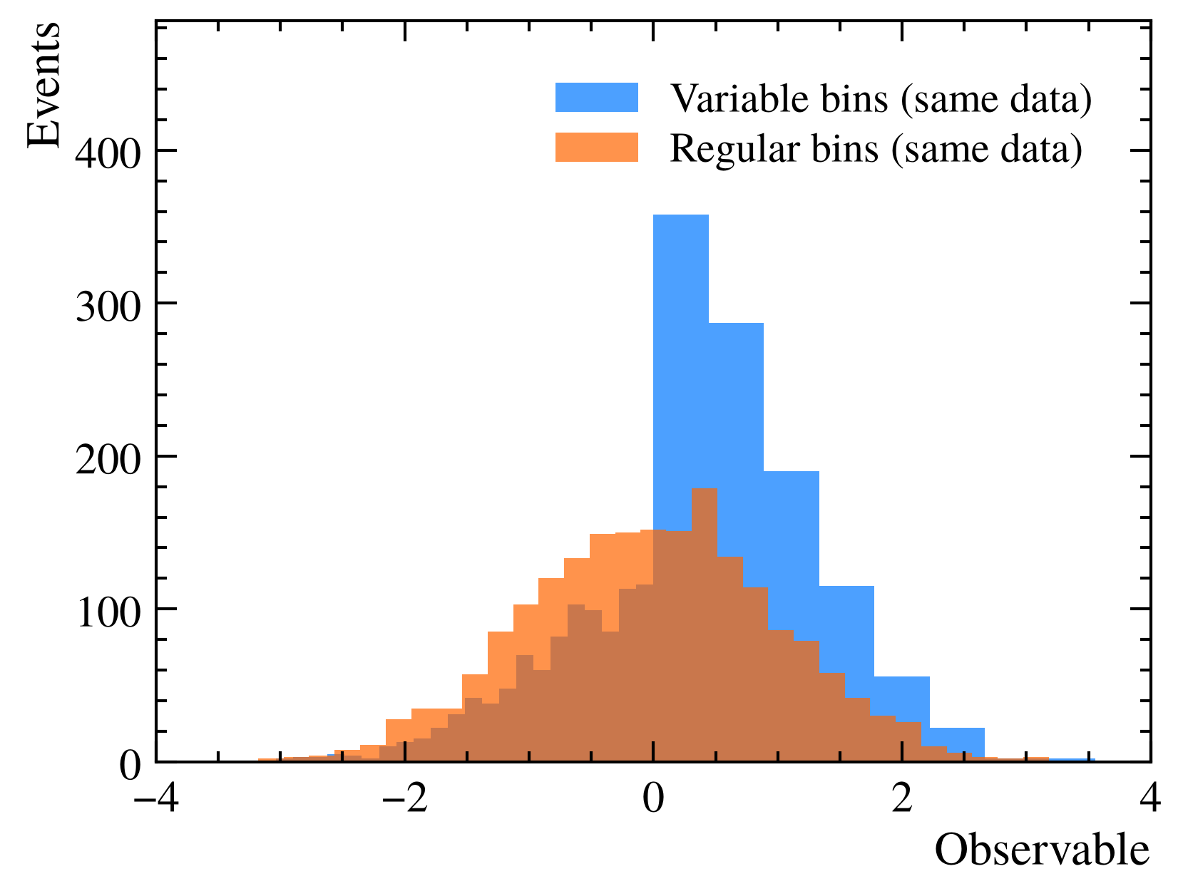
# Create histograms with different binning schemes
bins1 = np.r_[np.linspace(-4, 0, 30)[:-1], np.linspace(0, 4, 10)] # Variable binning
bins2 = np.linspace(-4, 4, 40) # Regular binning
h1 = hist.new.Var(bins1).Weight().fill(np.random.normal(0, 1, 2000))
h2 = hist.new.Var(bins2).Weight().fill(np.random.normal(0, 1, 2000))
# Plot
kwargs = {'density': True}
fig, ax = plt.subplots()
mh.histplot(h1, histtype='fill', alpha=0.7, label='Variable bins (same data)', ax=ax, **kwargs)
mh.histplot(h2, histtype='fill', alpha=0.7, label='Regular bins (same data)', ax=ax, **kwargs)
# Style
ax.set_xlabel('Observable')
ax.set_ylabel('Density')
ax.legend(loc='upper right')
mh.yscale_legend(soft_fail=True)
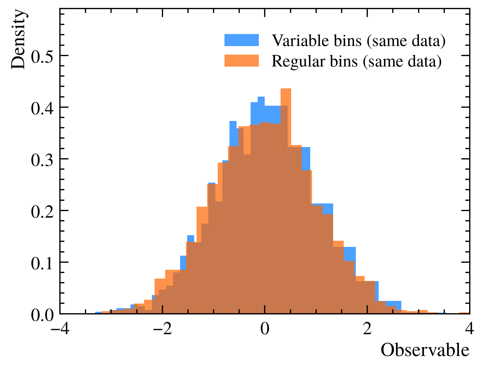
# Create histograms with different binning schemes
bins1 = np.r_[np.linspace(-4, 0, 30)[:-1], np.linspace(0, 4, 10)] # Variable binning
bins2 = np.linspace(-4, 4, 40) # Regular binning
h1 = hist.new.Var(bins1).Weight().fill(np.random.normal(0, 1, 2000))
h2 = hist.new.Var(bins2).Weight().fill(np.random.normal(0, 1, 2000))
# Plot
kwargs = {'binwnorm': True}
fig, ax = plt.subplots()
mh.histplot(h1, histtype='fill', alpha=0.7, label='Variable bins (same data)', ax=ax, **kwargs)
mh.histplot(h2, histtype='fill', alpha=0.7, label='Regular bins (same data)', ax=ax, **kwargs)
# Style
ax.set_xlabel('Observable')
ax.set_ylabel('Events / Bin Width')
ax.legend(loc='upper right')
mh.yscale_legend(soft_fail=True)
# Create histograms with different binning schemes
bins1 = np.r_[np.linspace(-4, 0, 30)[:-1], np.linspace(0, 4, 10)] # Variable binning
bins2 = np.linspace(-4, 4, 40) # Regular binning
h1 = hist.new.Var(bins1).Weight().fill(np.random.normal(0, 1, 2000))
h2 = hist.new.Var(bins2).Weight().fill(np.random.normal(0, 1, 2000))
# Plot
kwargs = {}
fig, ax = plt.subplots()
mh.histplot(h1, histtype='fill', alpha=0.7, label='Variable bins (same data)', ax=ax, **kwargs)
mh.histplot(h2, histtype='fill', alpha=0.7, label='Regular bins (same data)', ax=ax, **kwargs)
# Style
ax.set_xlabel('Observable')
ax.set_ylabel('Events')
ax.legend(loc='upper right')
mh.yscale_legend(soft_fail=True)
# Create histograms with different binning schemes
bins1 = np.r_[np.linspace(-4, 0, 30)[:-1], np.linspace(0, 4, 10)] # Variable binning
bins2 = np.linspace(-4, 4, 40) # Regular binning
h1 = hist.new.Var(bins1).Weight().fill(np.random.normal(0, 1, 2000))
h2 = hist.new.Var(bins2).Weight().fill(np.random.normal(0, 1, 2000))
# Plot
kwargs = {'density': True}
fig, ax = plt.subplots()
mh.histplot(h1, histtype='fill', alpha=0.7, label='Variable bins (same data)', ax=ax, **kwargs)
mh.histplot(h2, histtype='fill', alpha=0.7, label='Regular bins (same data)', ax=ax, **kwargs)
# Style
ax.set_xlabel('Observable')
ax.set_ylabel('Density')
ax.legend(loc='upper right')
mh.yscale_legend(soft_fail=True)
# Create histograms with different binning schemes
bins1 = np.r_[np.linspace(-4, 0, 30)[:-1], np.linspace(0, 4, 10)] # Variable binning
bins2 = np.linspace(-4, 4, 40) # Regular binning
h1 = hist.new.Var(bins1).Weight().fill(np.random.normal(0, 1, 2000))
h2 = hist.new.Var(bins2).Weight().fill(np.random.normal(0, 1, 2000))
# Plot
kwargs = {'binwnorm': True}
fig, ax = plt.subplots()
mh.histplot(h1, histtype='fill', alpha=0.7, label='Variable bins (same data)', ax=ax, **kwargs)
mh.histplot(h2, histtype='fill', alpha=0.7, label='Regular bins (same data)', ax=ax, **kwargs)
# Style
ax.set_xlabel('Observable')
ax.set_ylabel('Events / Bin Width')
ax.legend(loc='upper right')
mh.yscale_legend(soft_fail=True)
# Create histograms with different binning schemes
bins1 = np.r_[np.linspace(-4, 0, 30)[:-1], np.linspace(0, 4, 10)] # Variable binning
bins2 = np.linspace(-4, 4, 40) # Regular binning
h1 = hist.new.Var(bins1).Weight().fill(np.random.normal(0, 1, 2000))
h2 = hist.new.Var(bins2).Weight().fill(np.random.normal(0, 1, 2000))
# Plot
kwargs = {}
fig, ax = plt.subplots()
mh.histplot(h1, histtype='fill', alpha=0.7, label='Variable bins (same data)', ax=ax, **kwargs)
mh.histplot(h2, histtype='fill', alpha=0.7, label='Regular bins (same data)', ax=ax, **kwargs)
# Style
ax.set_xlabel('Observable')
ax.set_ylabel('Events')
ax.legend(loc='upper right')
mh.yscale_legend(soft_fail=True)
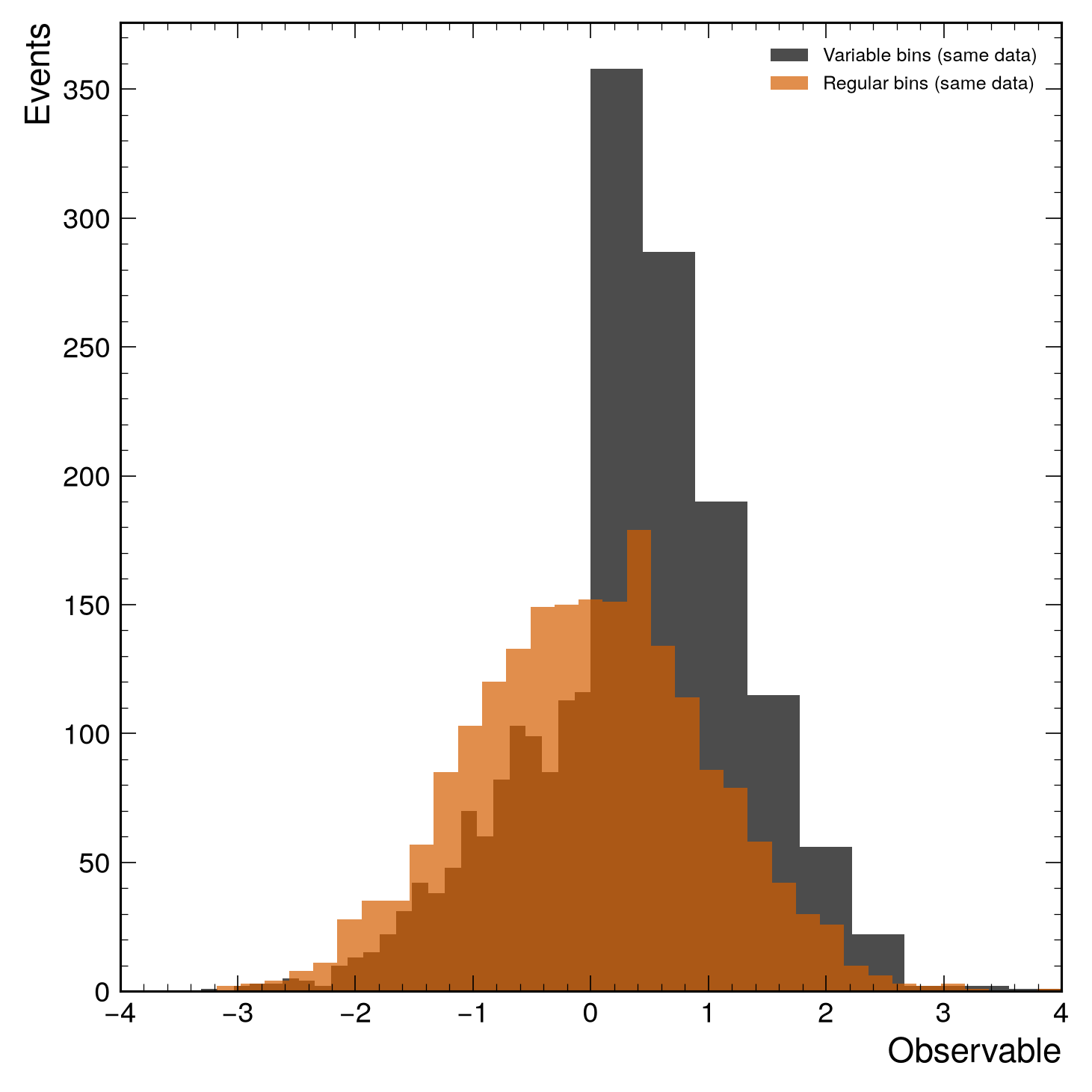
# Create histograms with different binning schemes
bins1 = np.r_[np.linspace(-4, 0, 30)[:-1], np.linspace(0, 4, 10)] # Variable binning
bins2 = np.linspace(-4, 4, 40) # Regular binning
h1 = hist.new.Var(bins1).Weight().fill(np.random.normal(0, 1, 2000))
h2 = hist.new.Var(bins2).Weight().fill(np.random.normal(0, 1, 2000))
# Plot
kwargs = {'density': True}
fig, ax = plt.subplots()
mh.histplot(h1, histtype='fill', alpha=0.7, label='Variable bins (same data)', ax=ax, **kwargs)
mh.histplot(h2, histtype='fill', alpha=0.7, label='Regular bins (same data)', ax=ax, **kwargs)
# Style
ax.set_xlabel('Observable')
ax.set_ylabel('Density')
ax.legend(loc='upper right')
mh.yscale_legend(soft_fail=True)
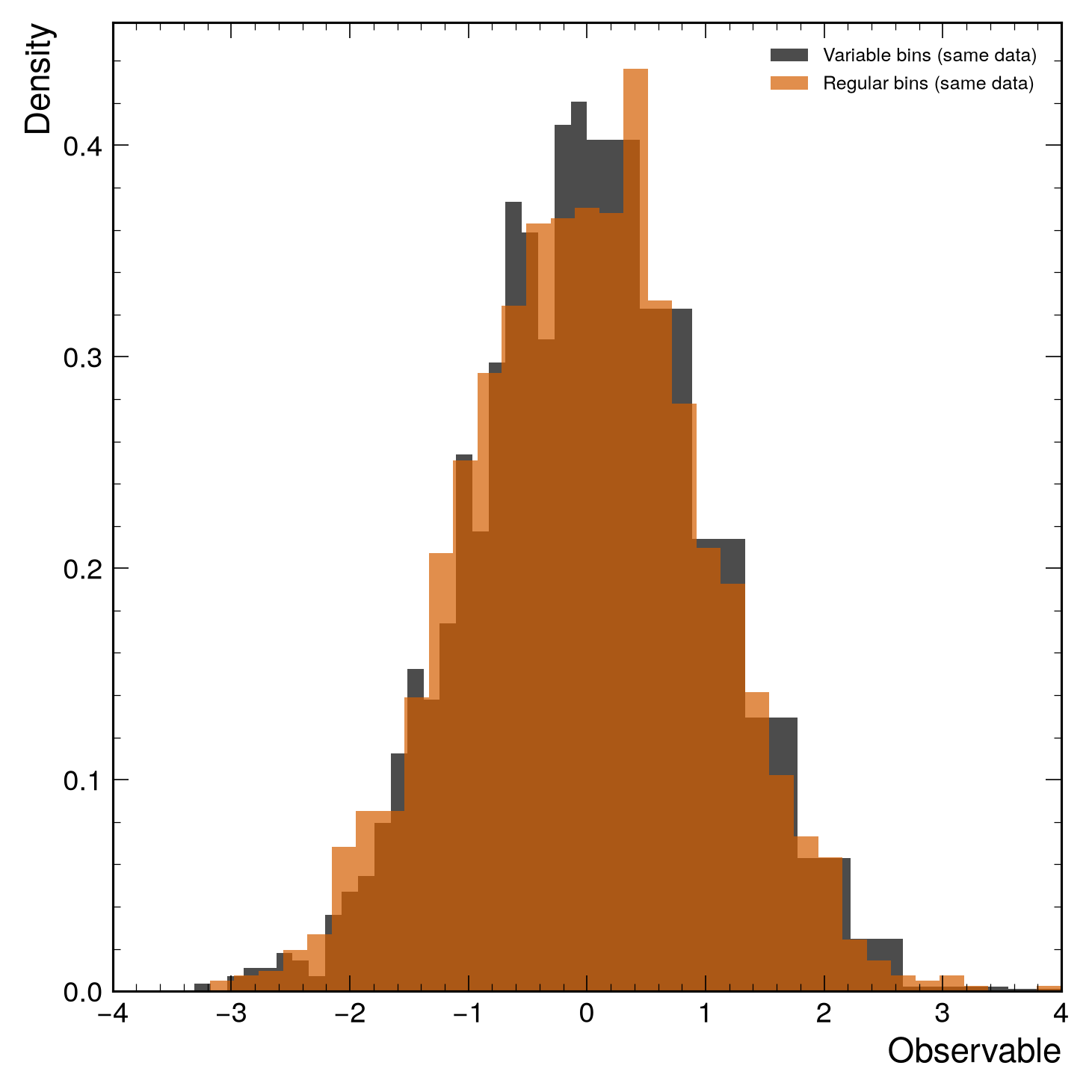
# Create histograms with different binning schemes
bins1 = np.r_[np.linspace(-4, 0, 30)[:-1], np.linspace(0, 4, 10)] # Variable binning
bins2 = np.linspace(-4, 4, 40) # Regular binning
h1 = hist.new.Var(bins1).Weight().fill(np.random.normal(0, 1, 2000))
h2 = hist.new.Var(bins2).Weight().fill(np.random.normal(0, 1, 2000))
# Plot
kwargs = {'binwnorm': True}
fig, ax = plt.subplots()
mh.histplot(h1, histtype='fill', alpha=0.7, label='Variable bins (same data)', ax=ax, **kwargs)
mh.histplot(h2, histtype='fill', alpha=0.7, label='Regular bins (same data)', ax=ax, **kwargs)
# Style
ax.set_xlabel('Observable')
ax.set_ylabel('Events / Bin Width')
ax.legend(loc='upper right')
mh.yscale_legend(soft_fail=True)
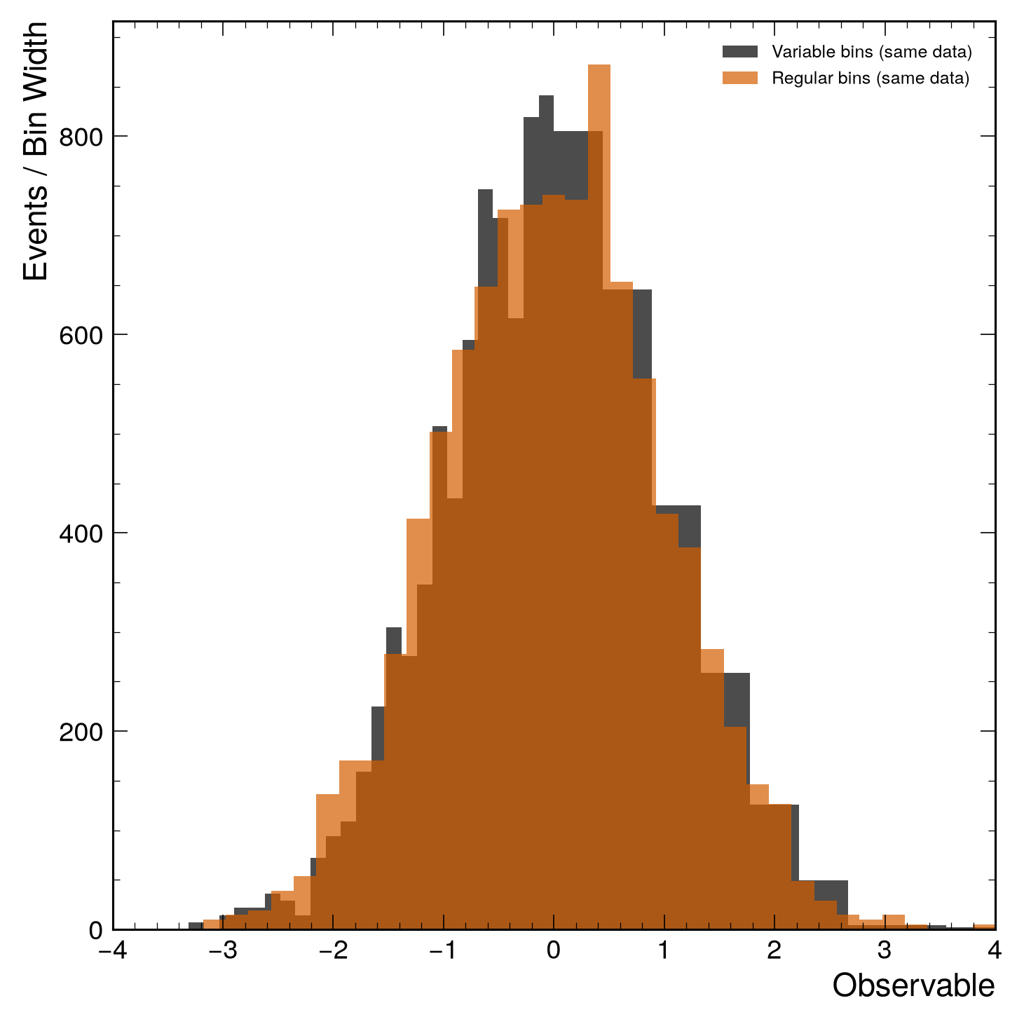
2D Histograms¤
Use mh.hist2dplot() for 2D histogram visualization: